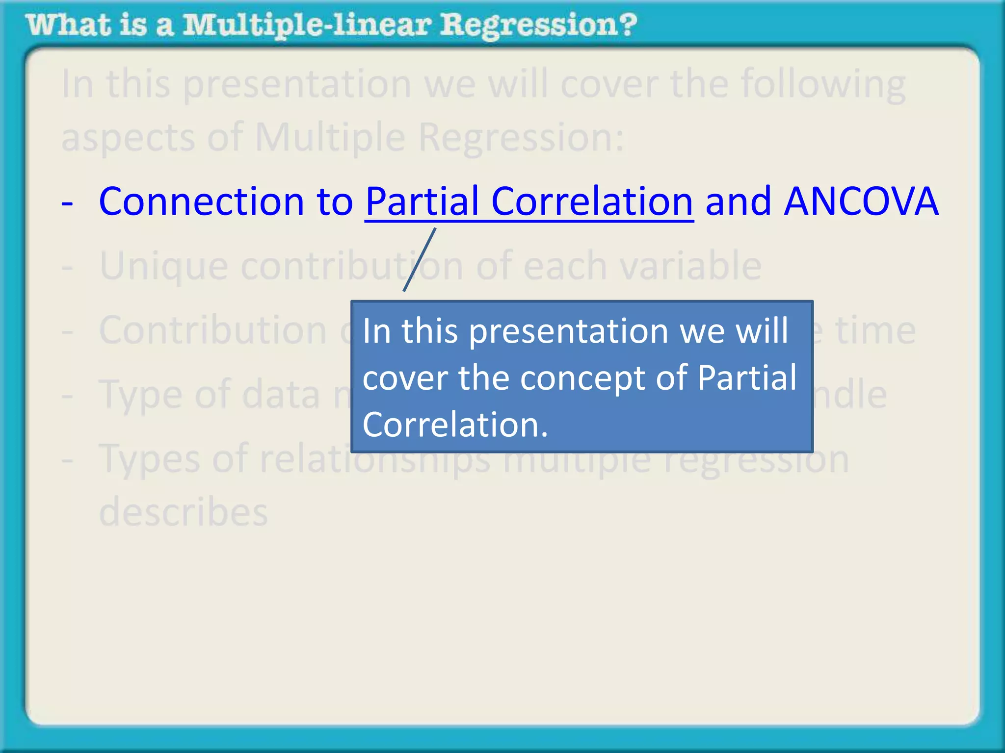
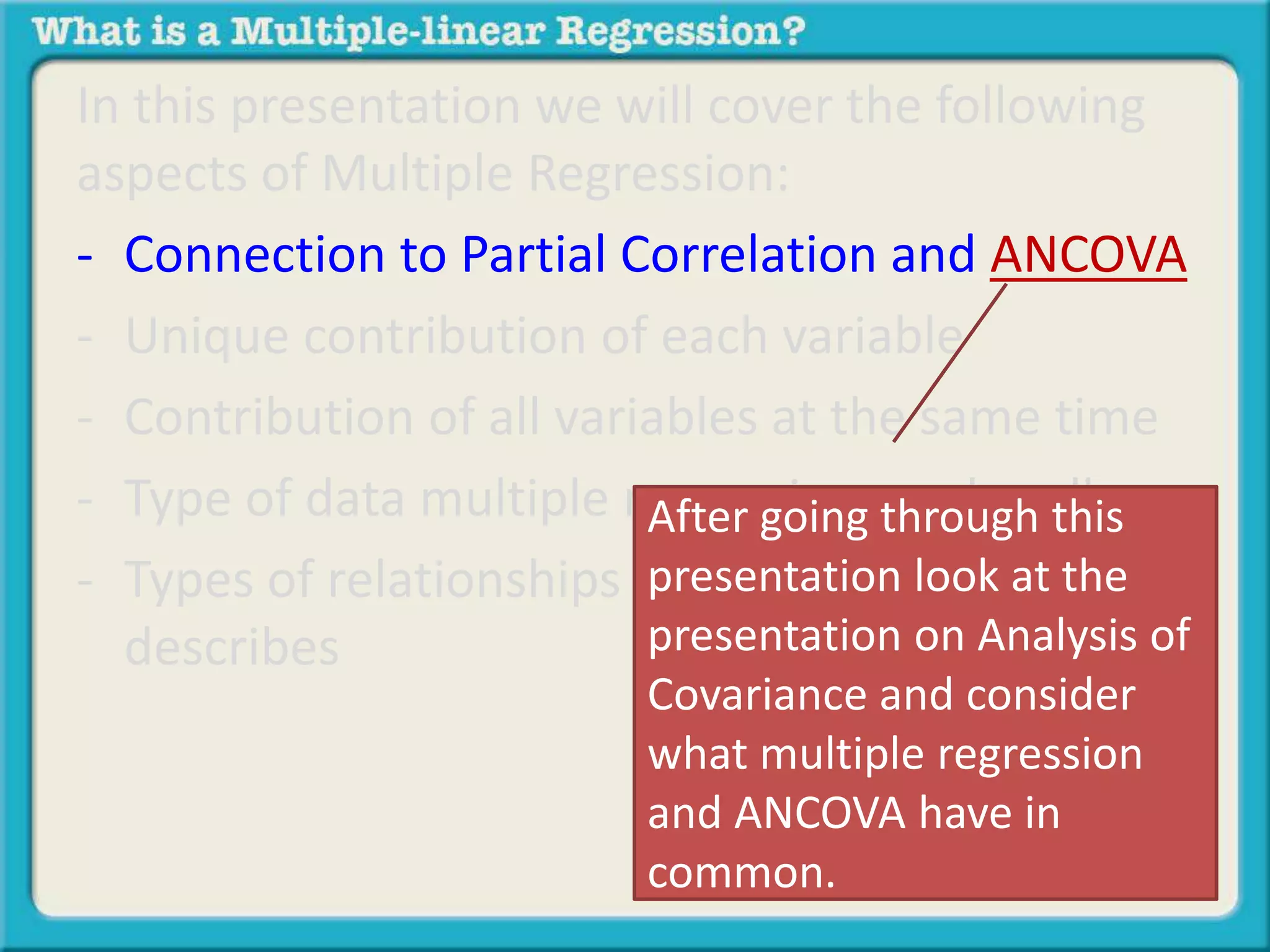
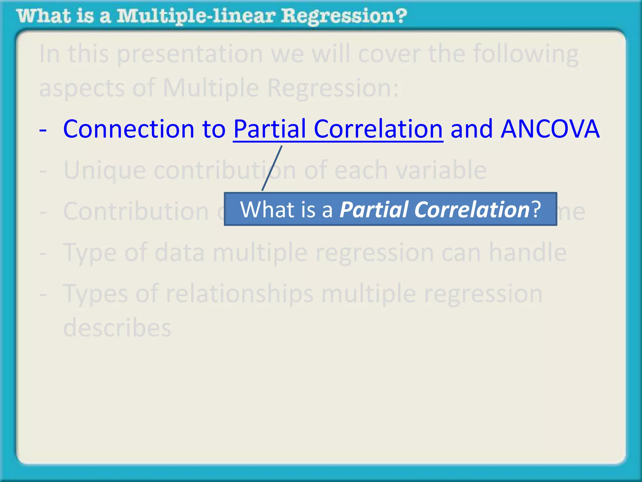
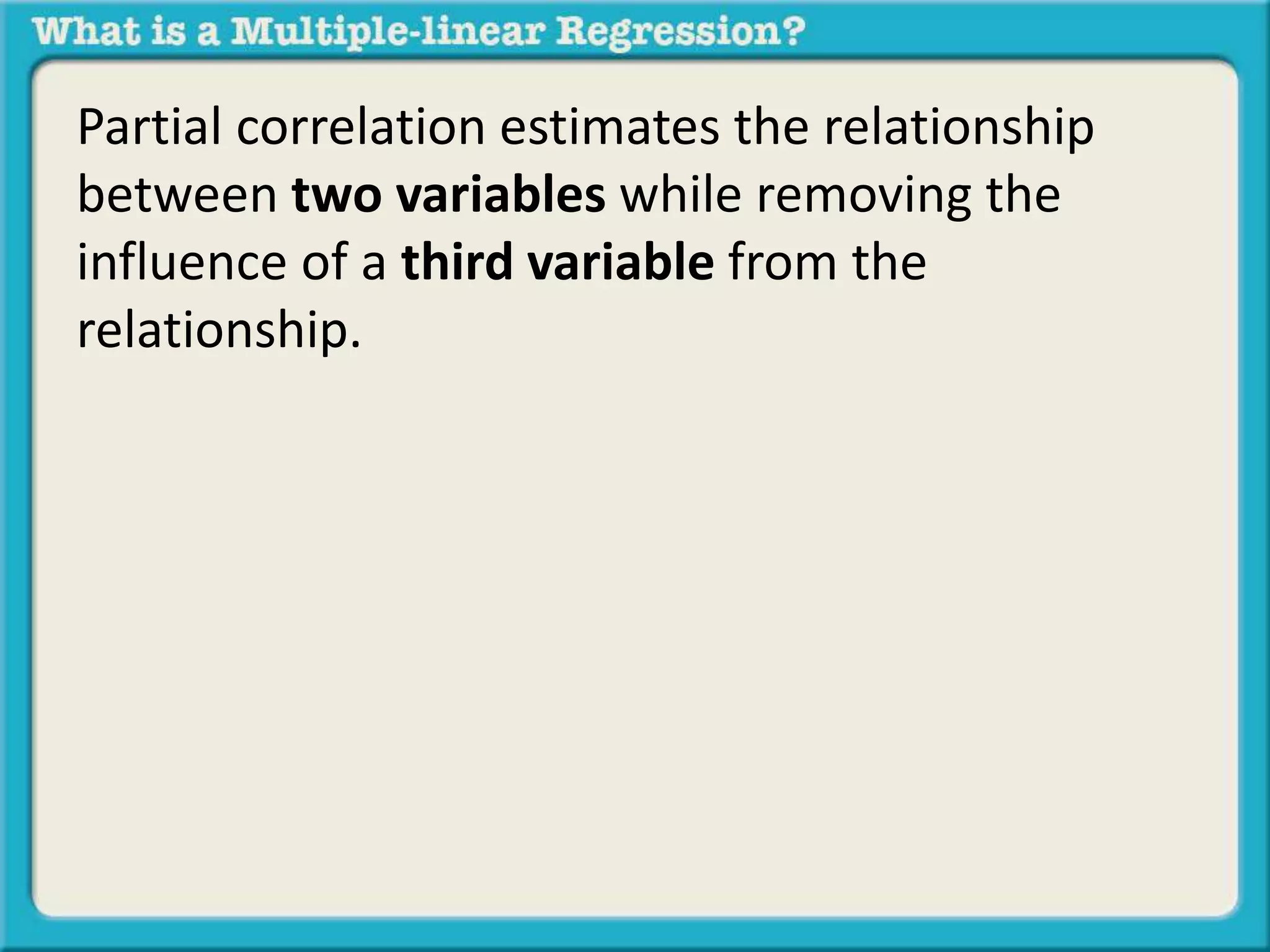
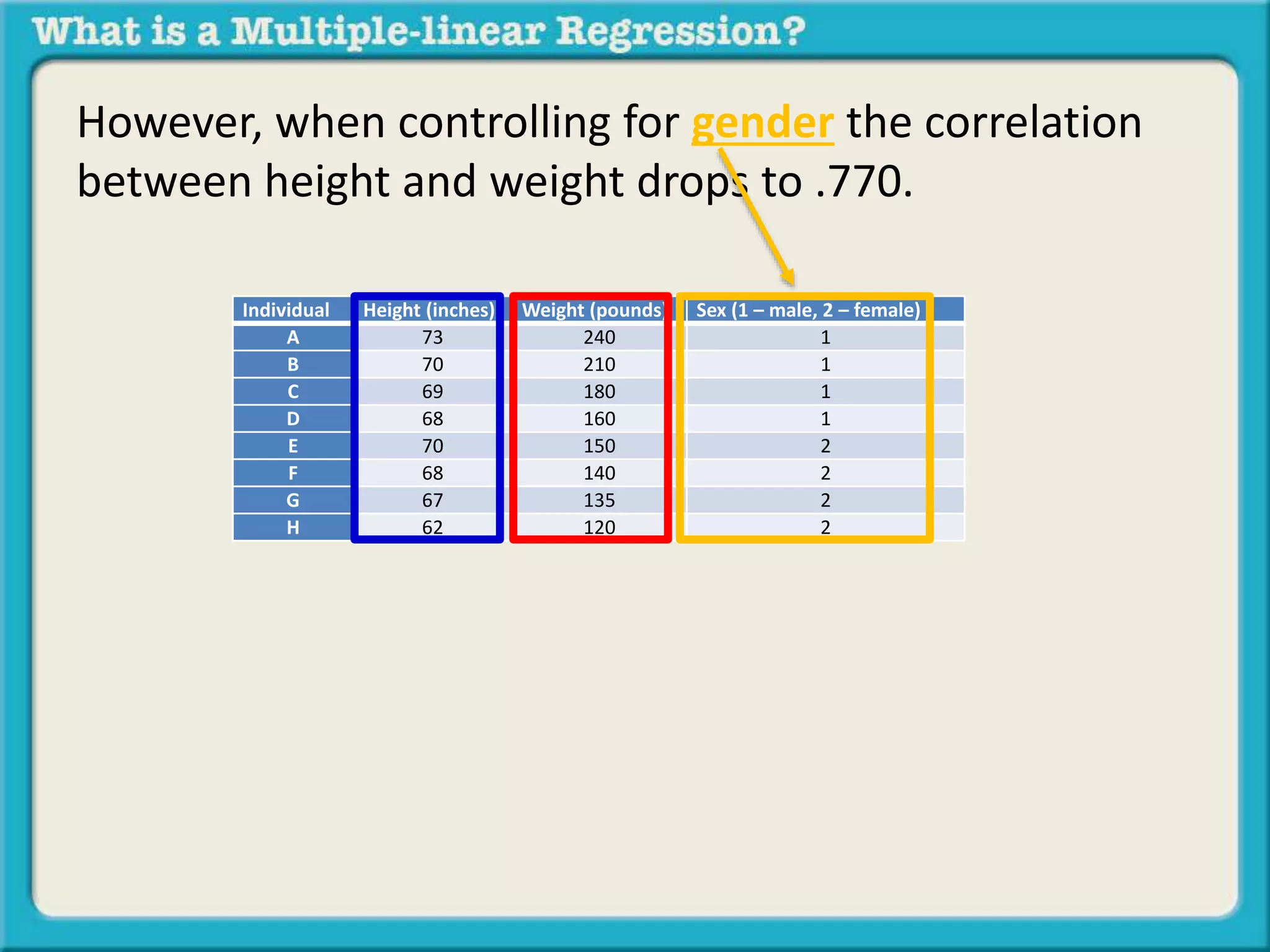
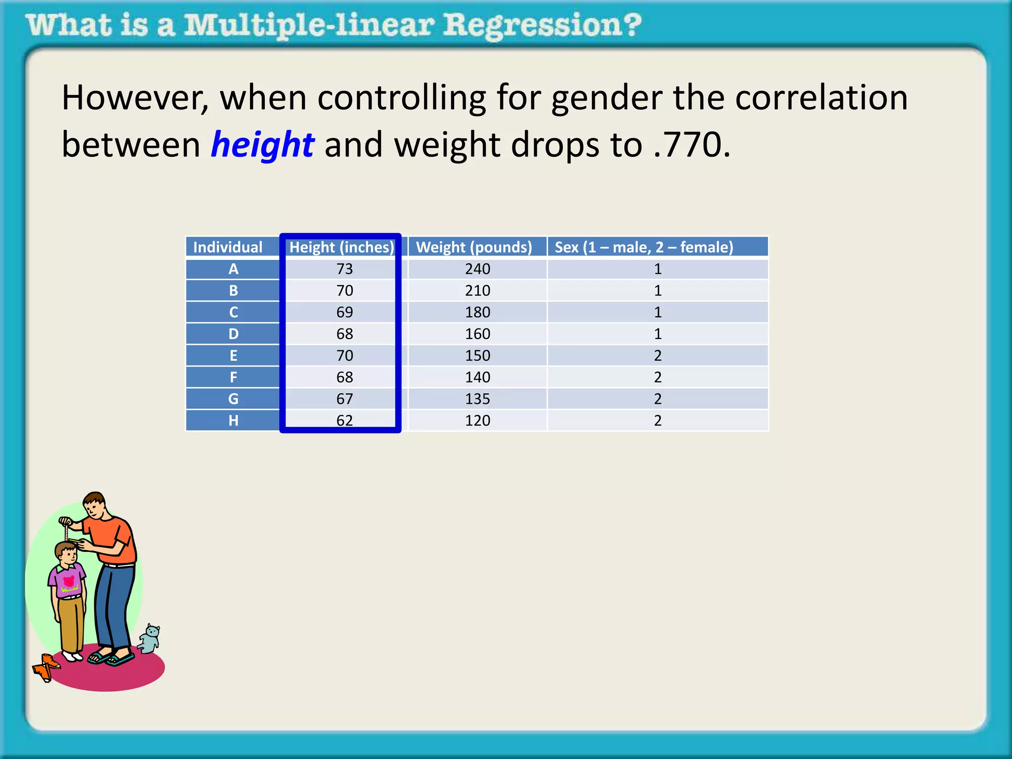
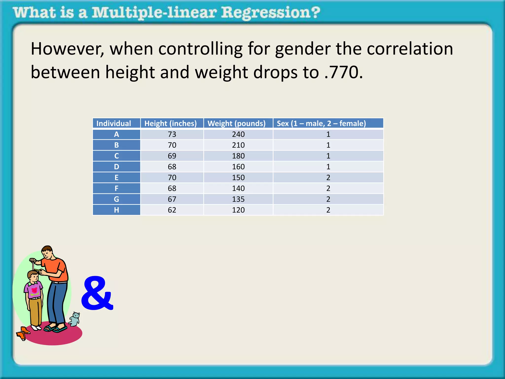
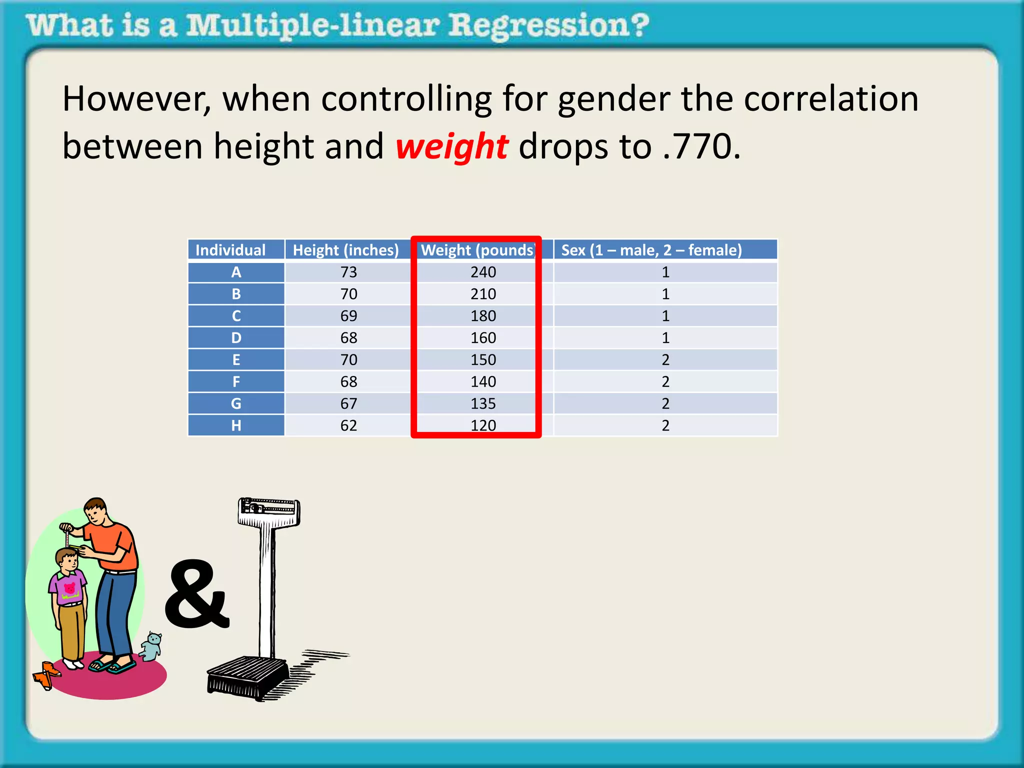
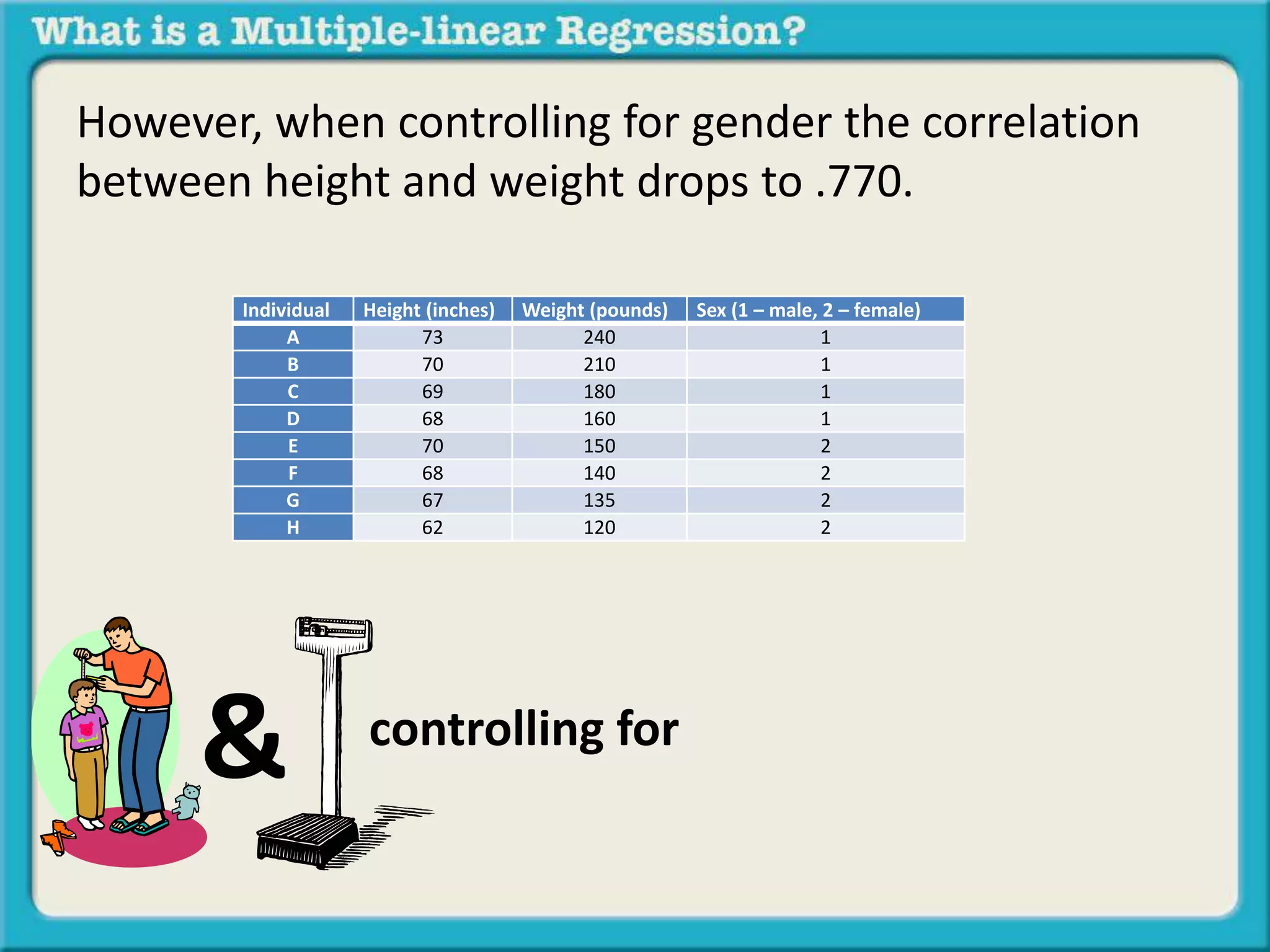
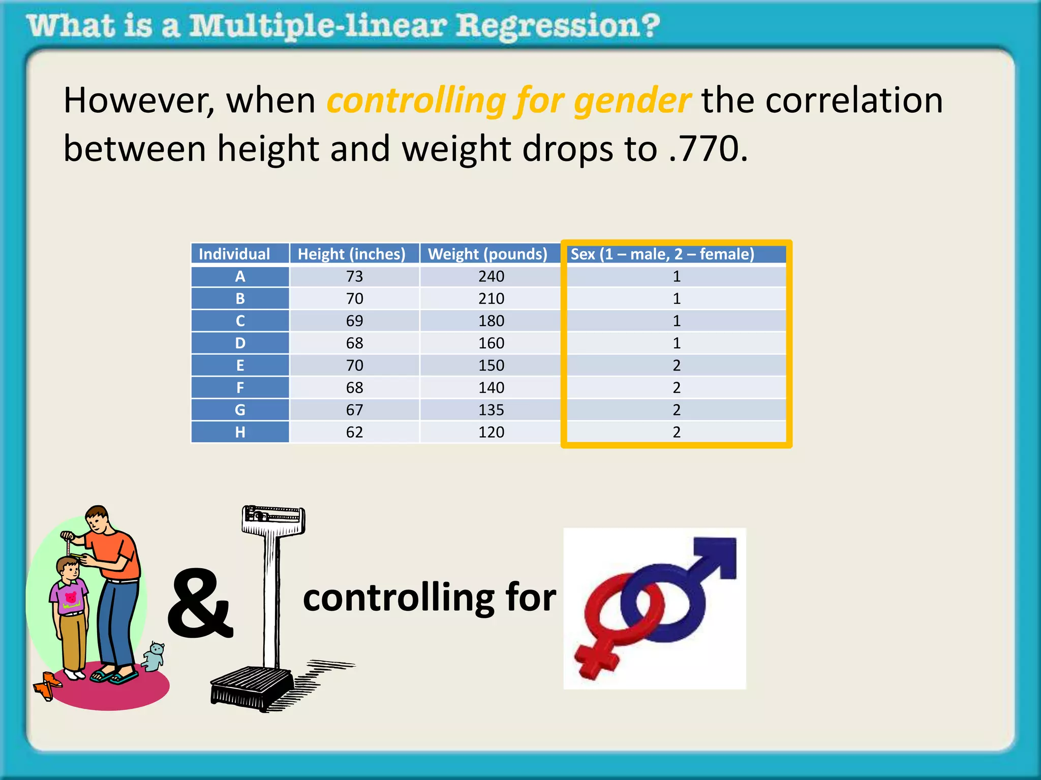
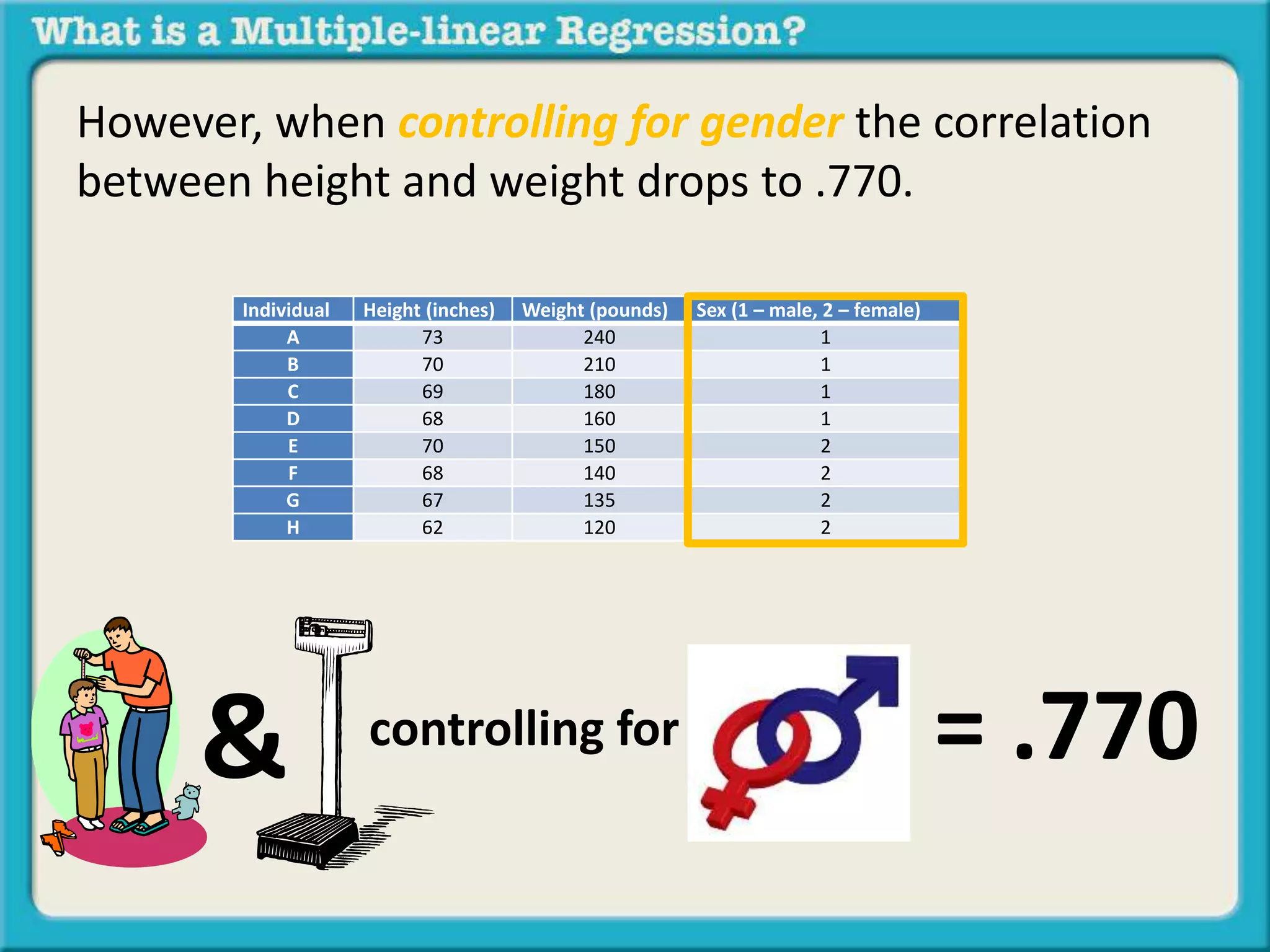
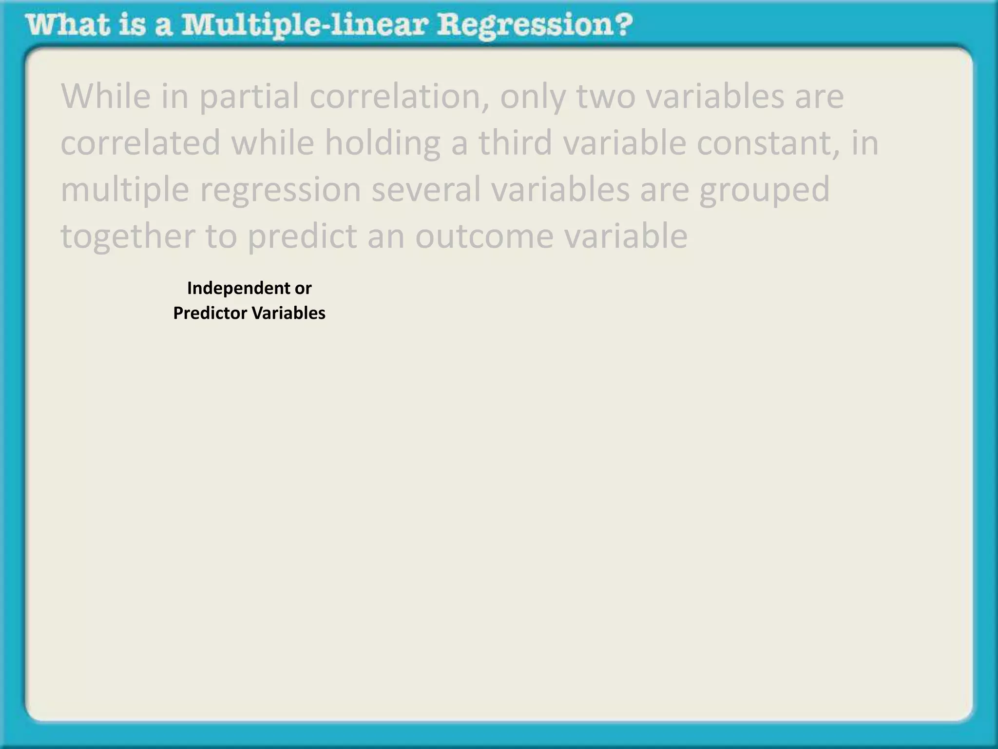
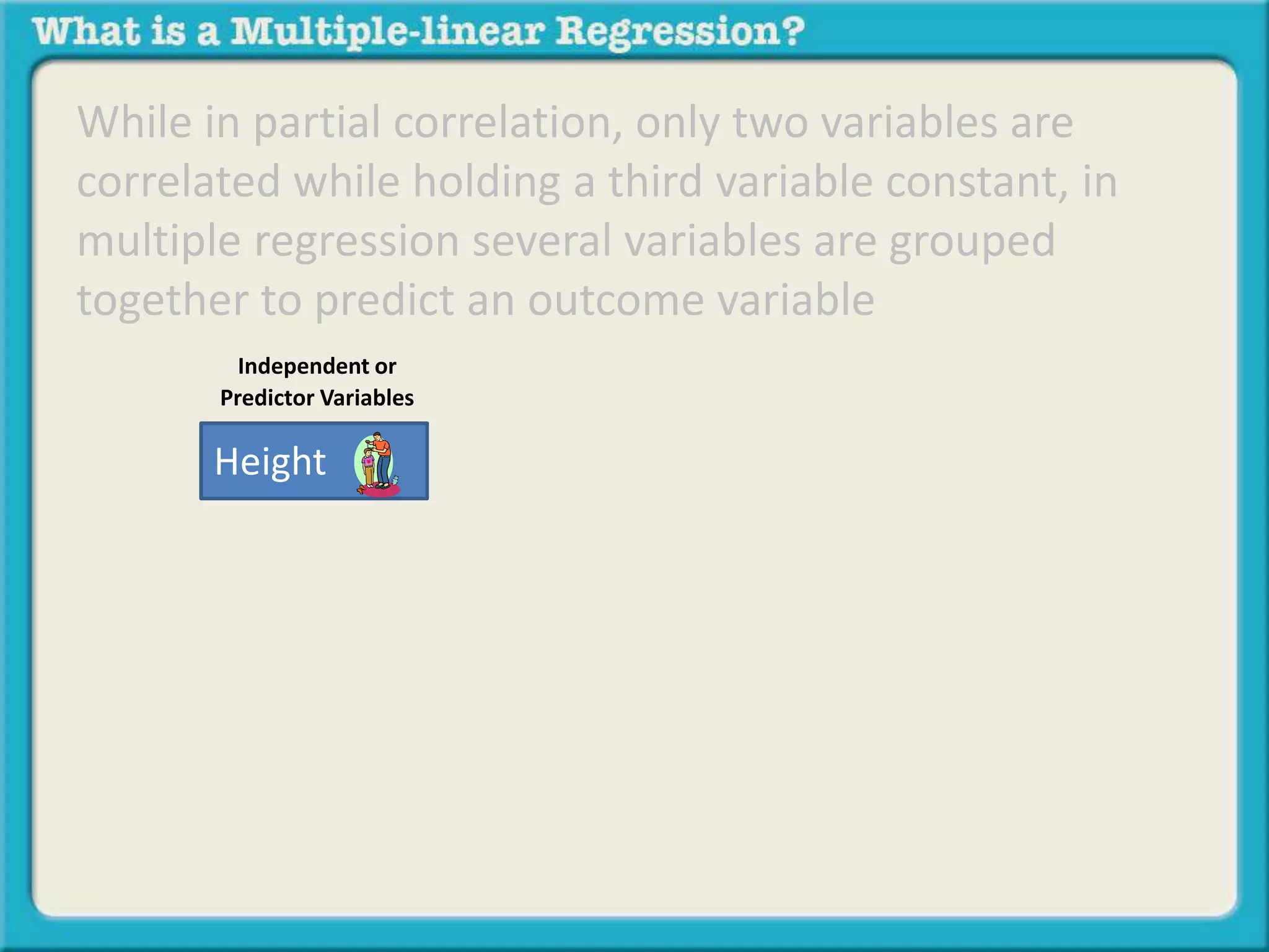
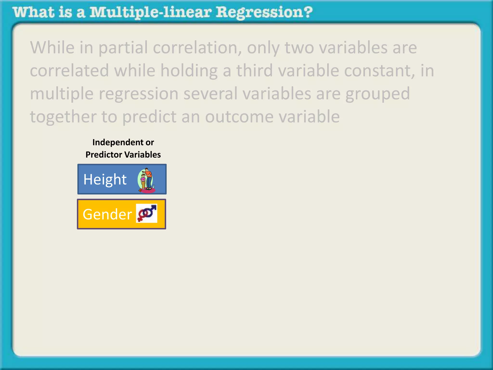
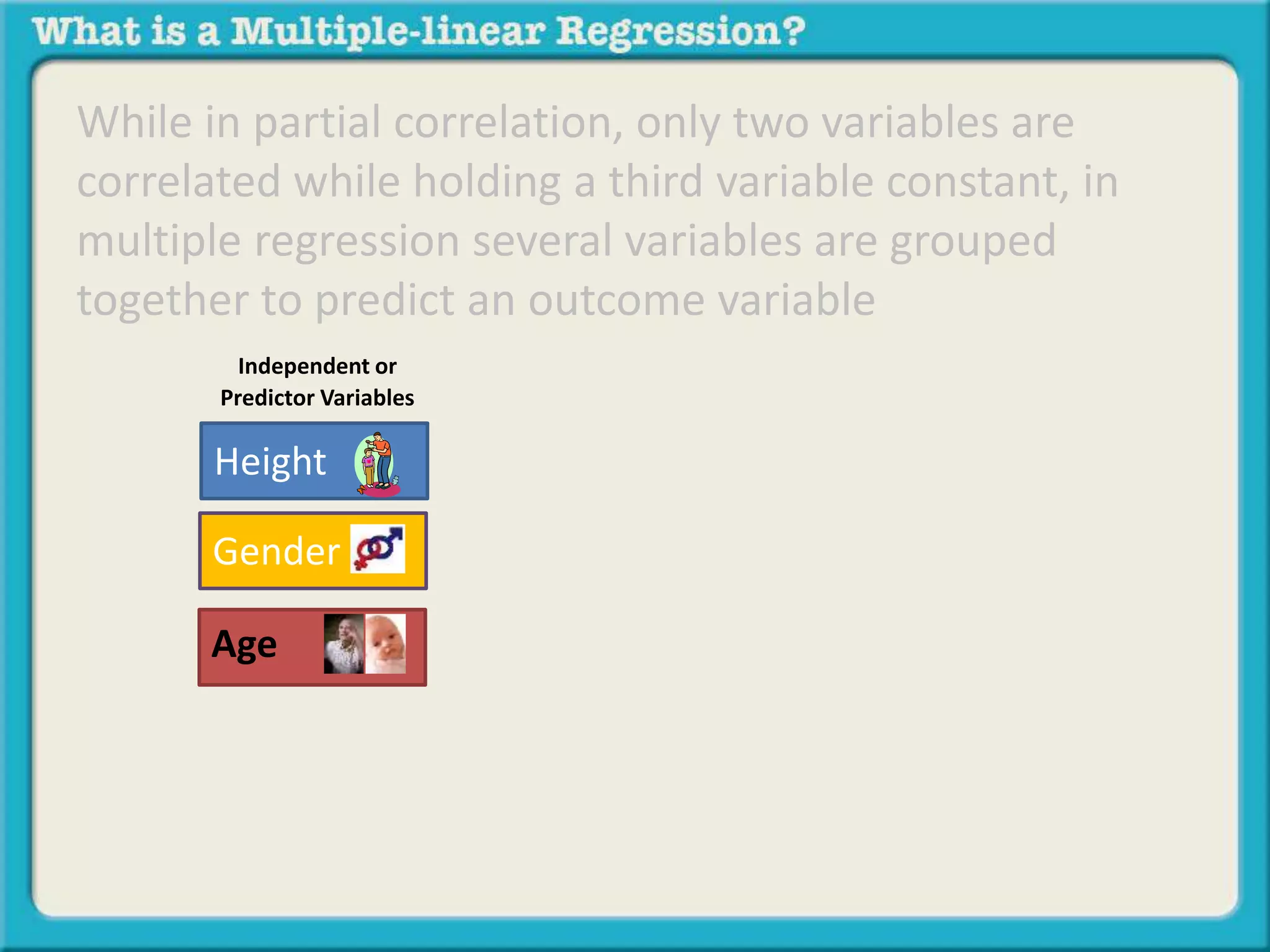
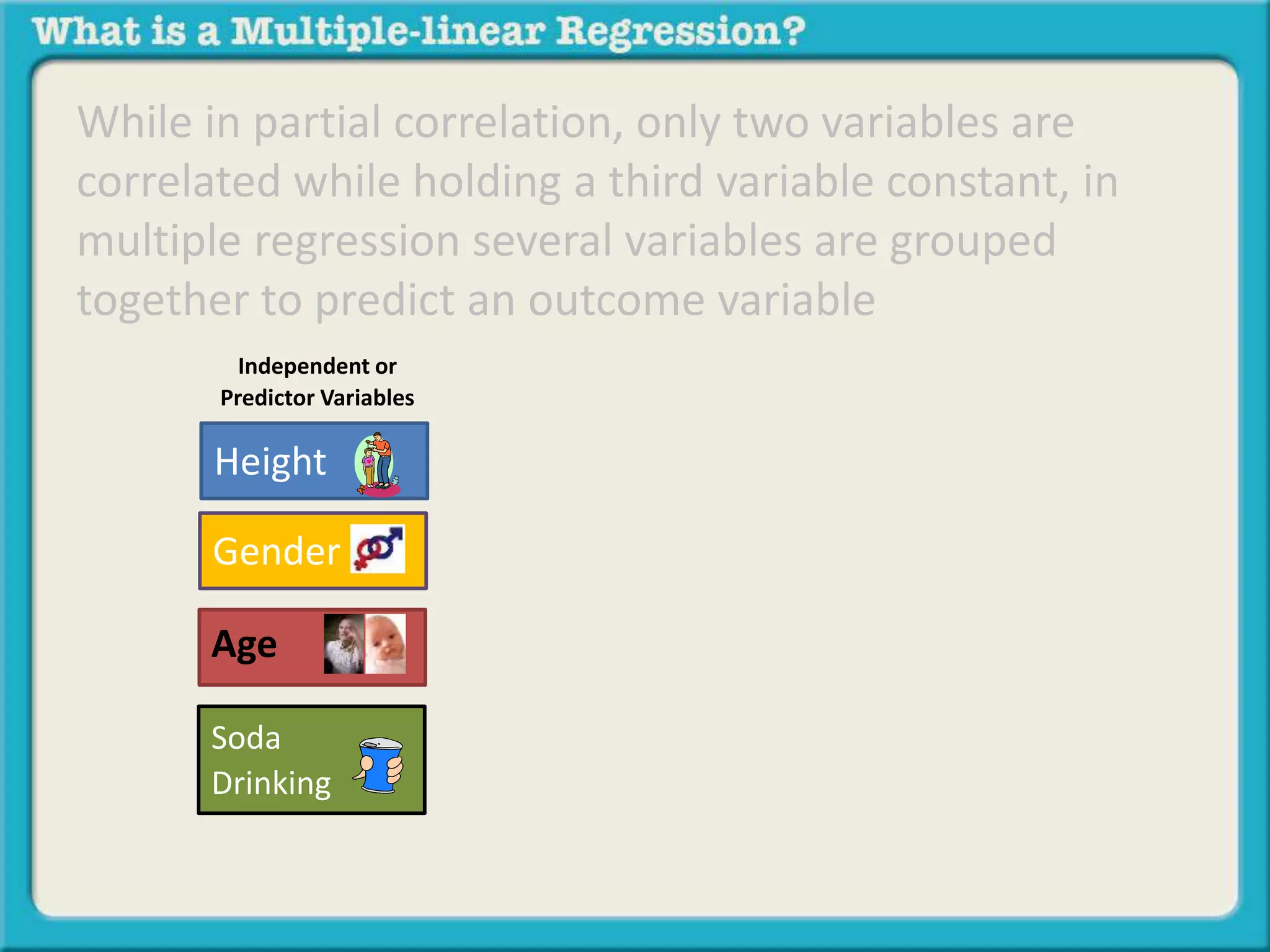
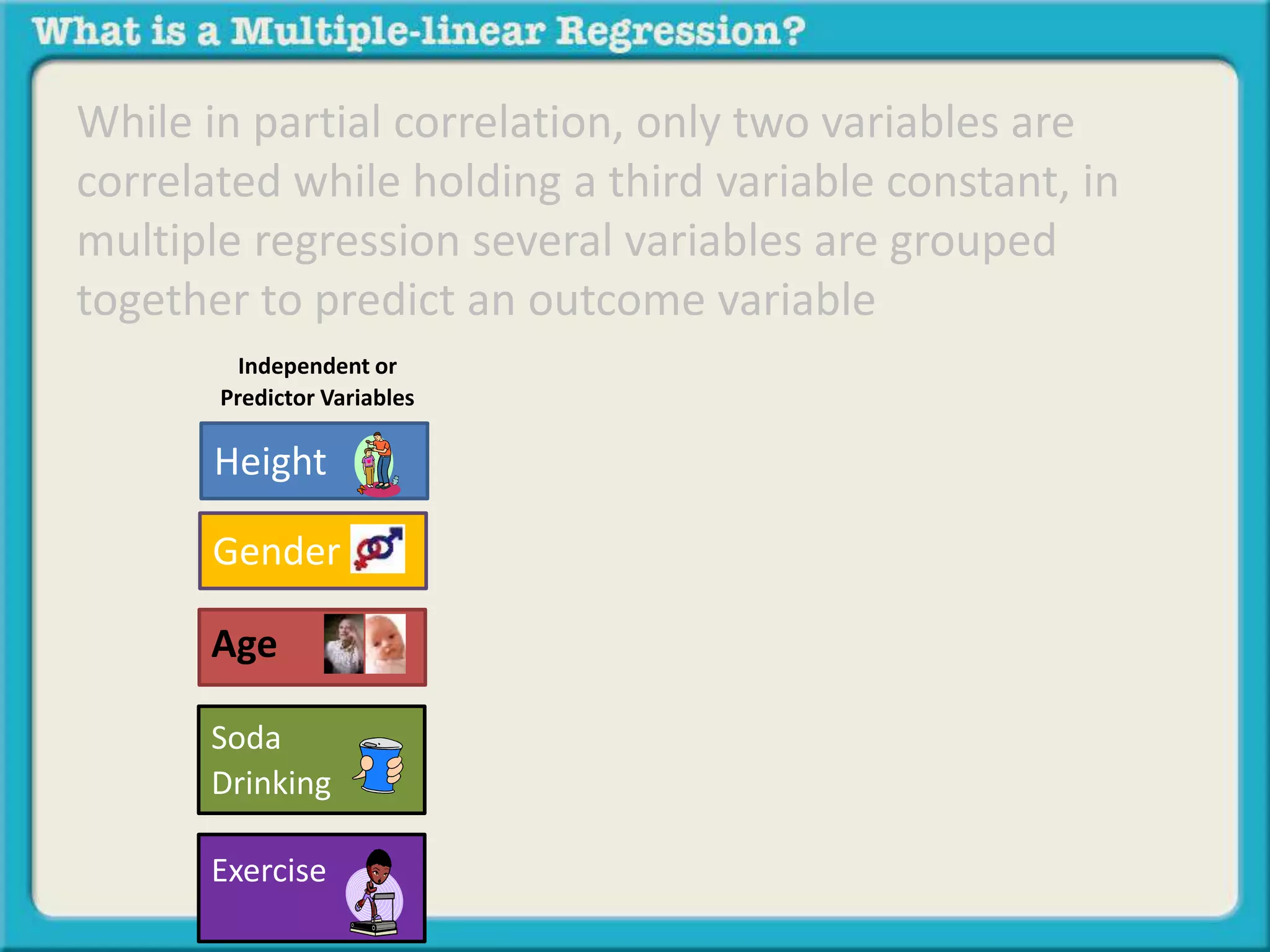
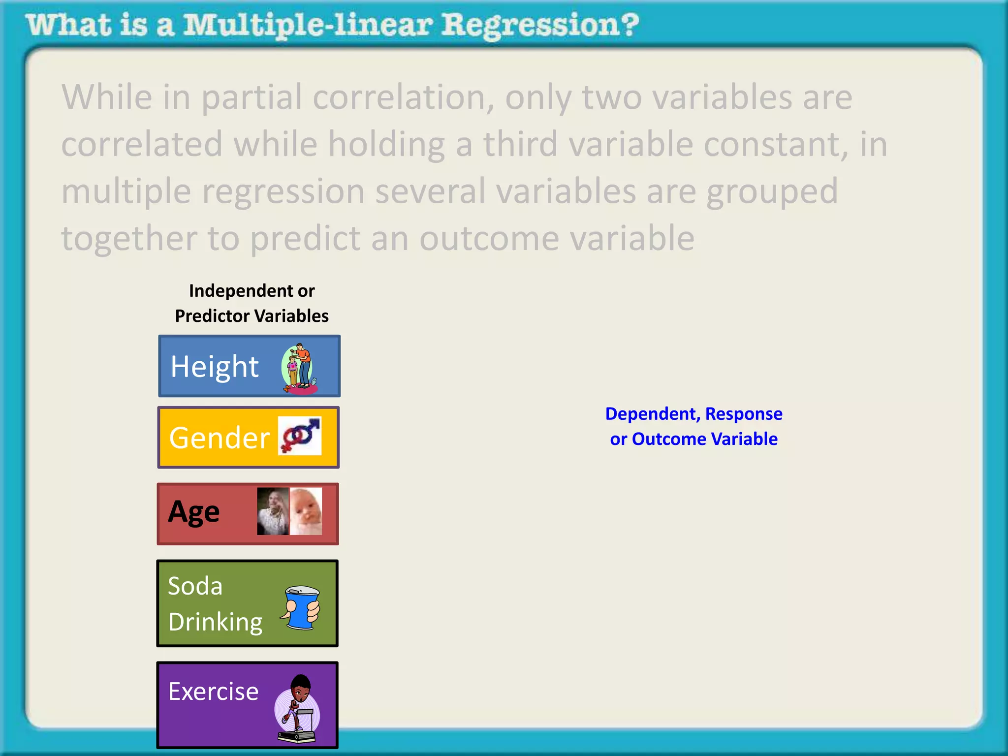
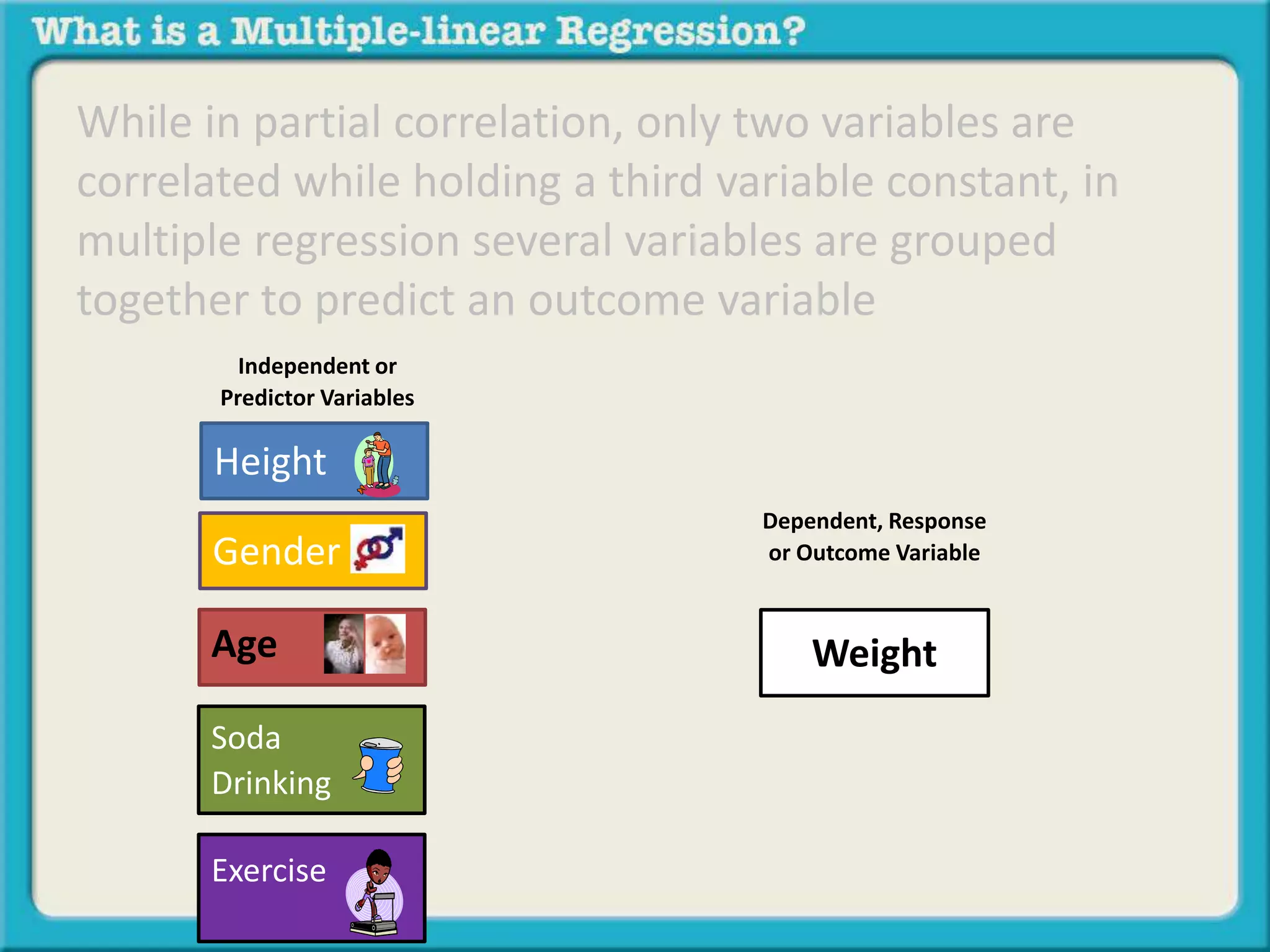
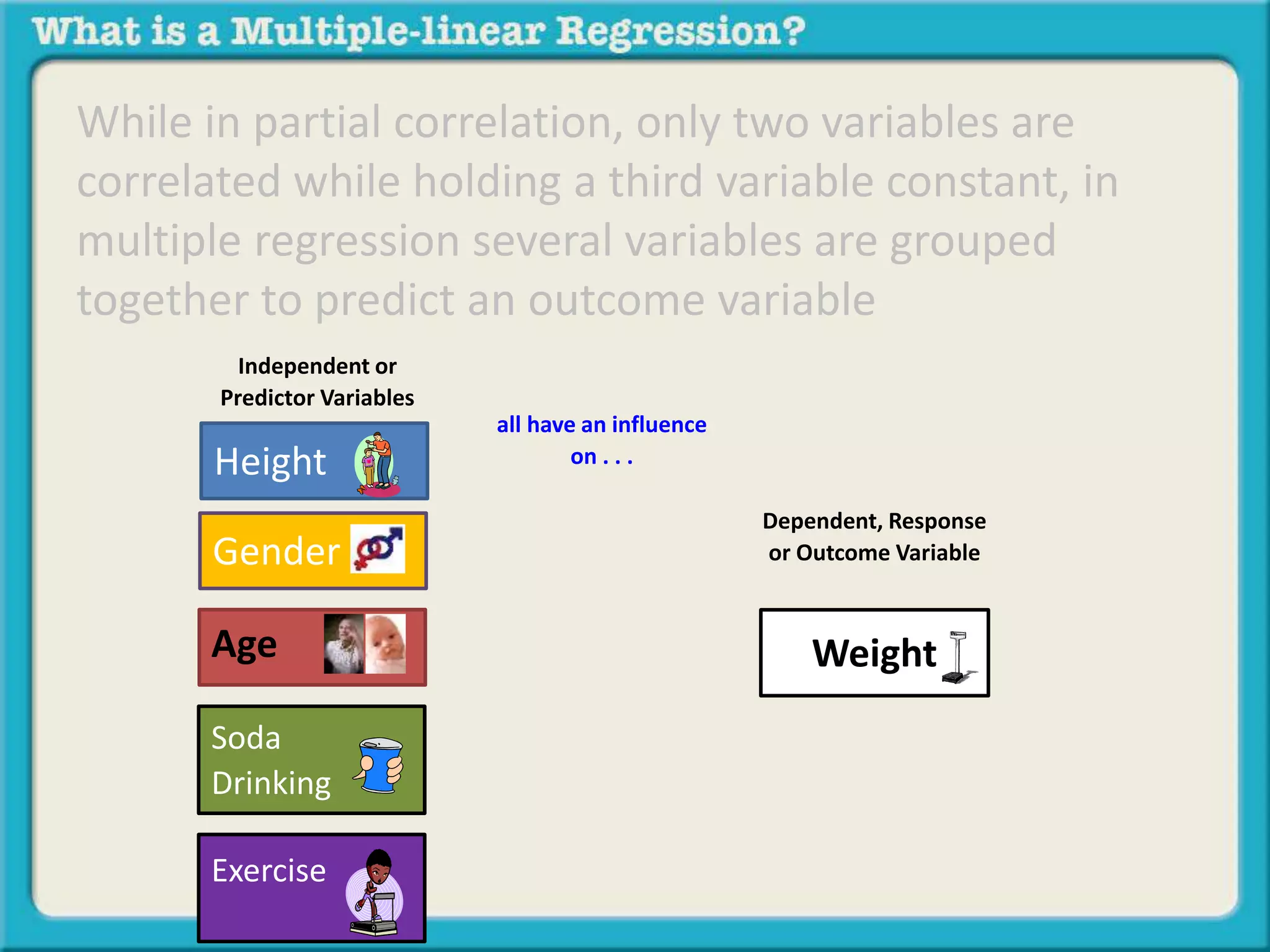
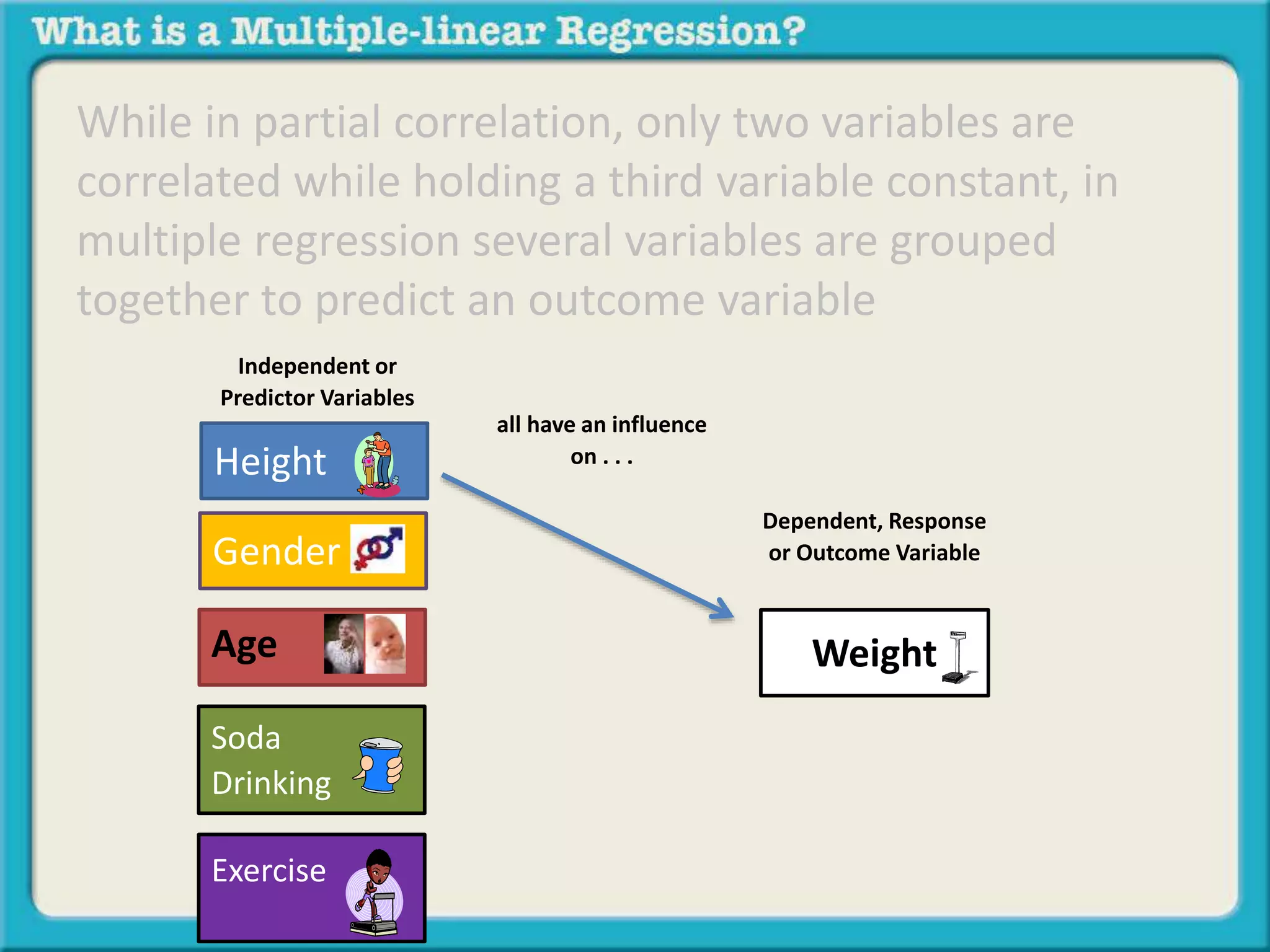
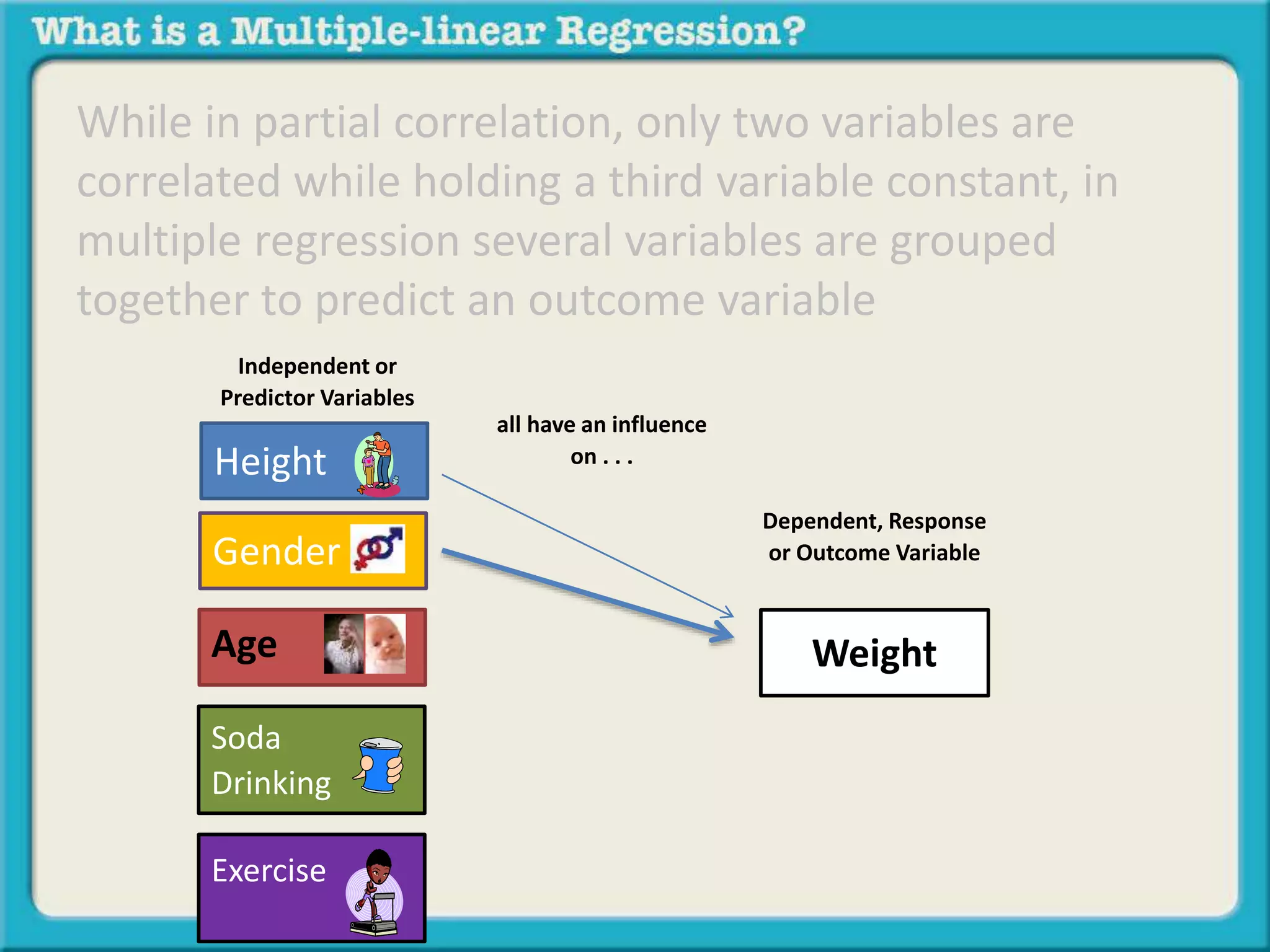
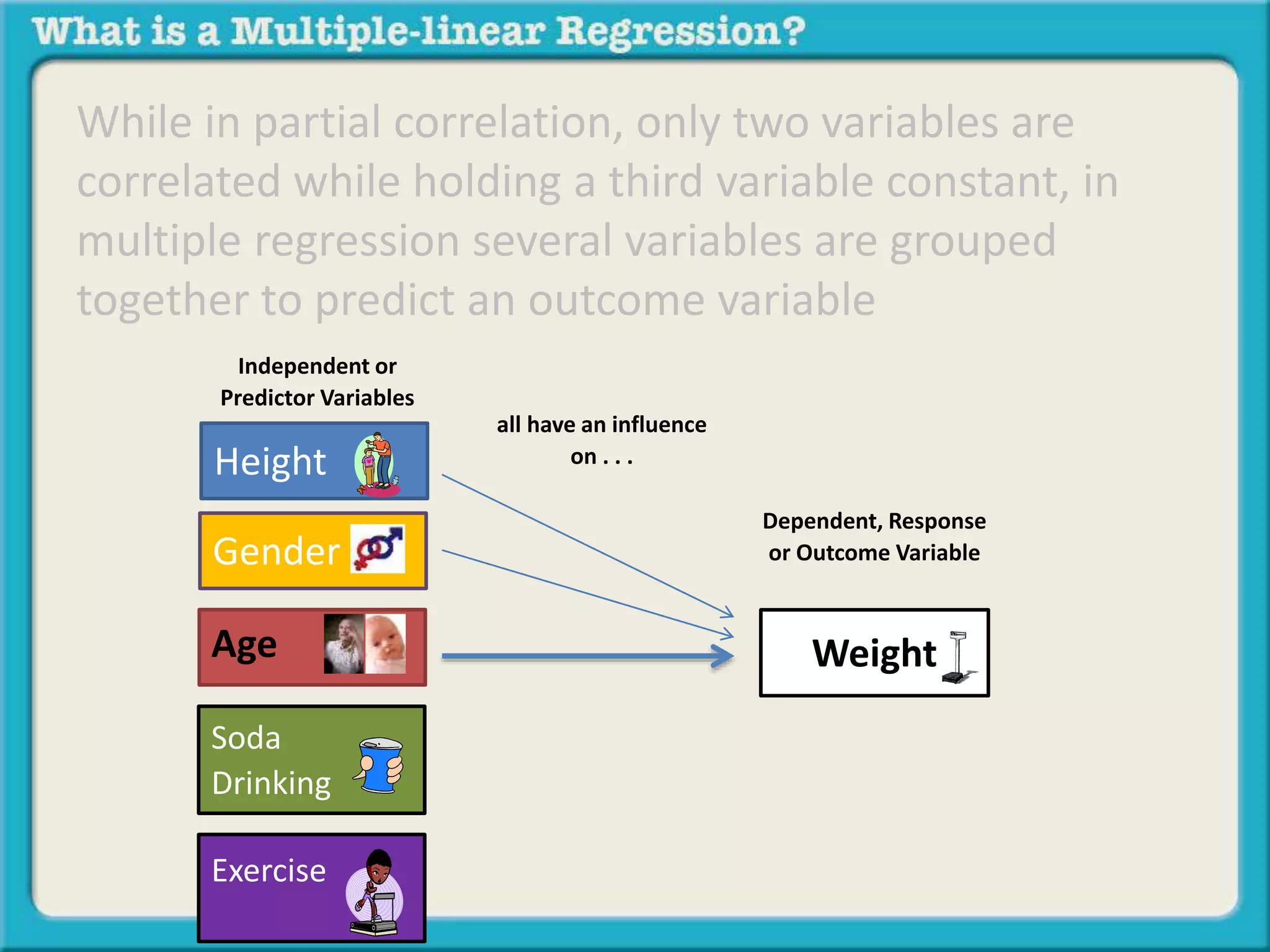
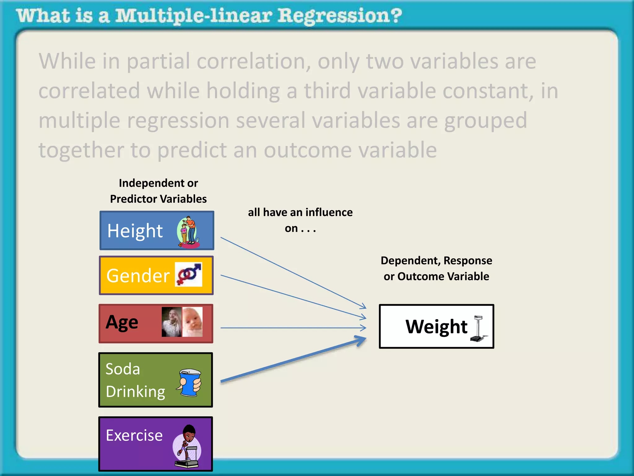
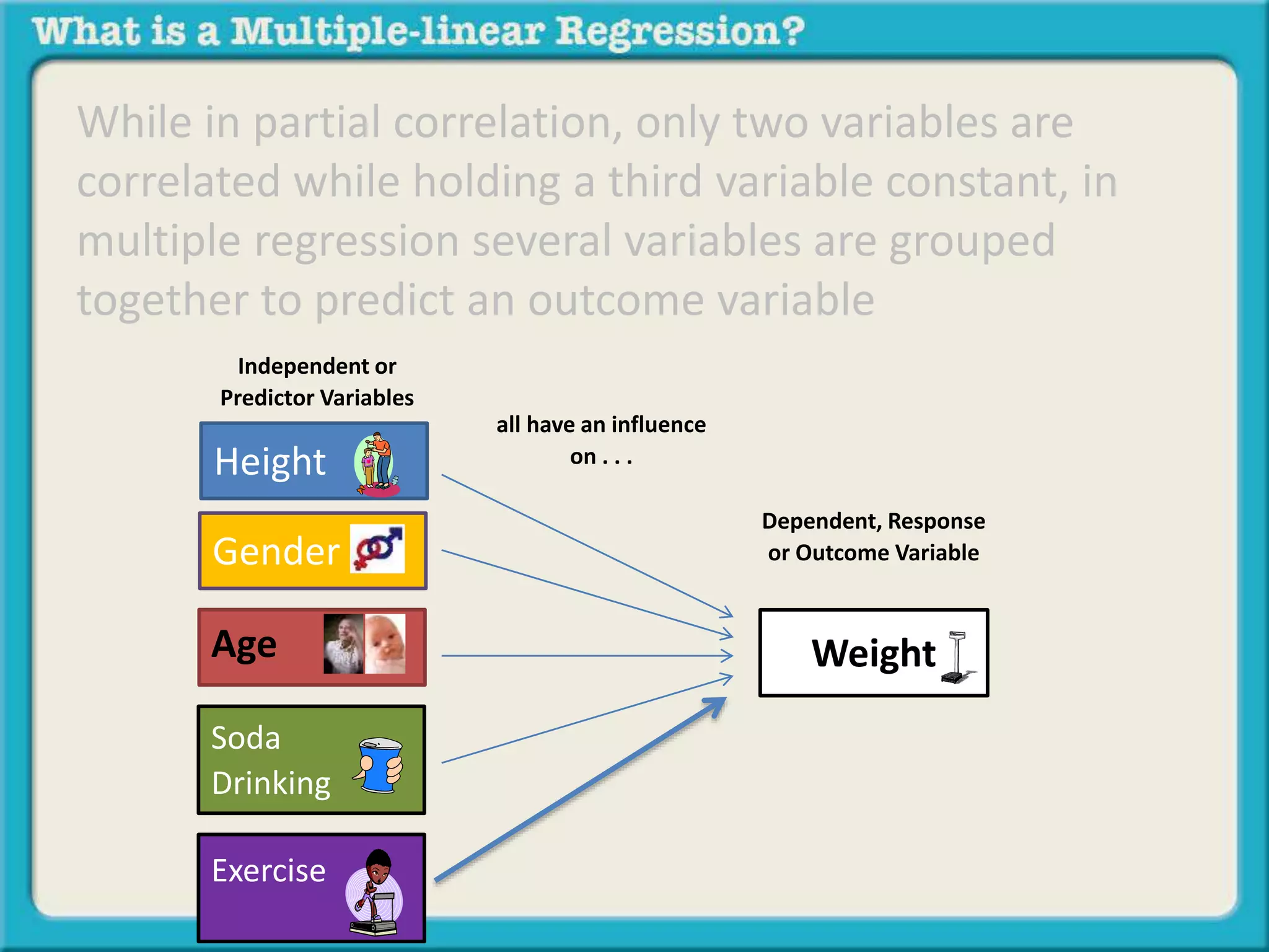
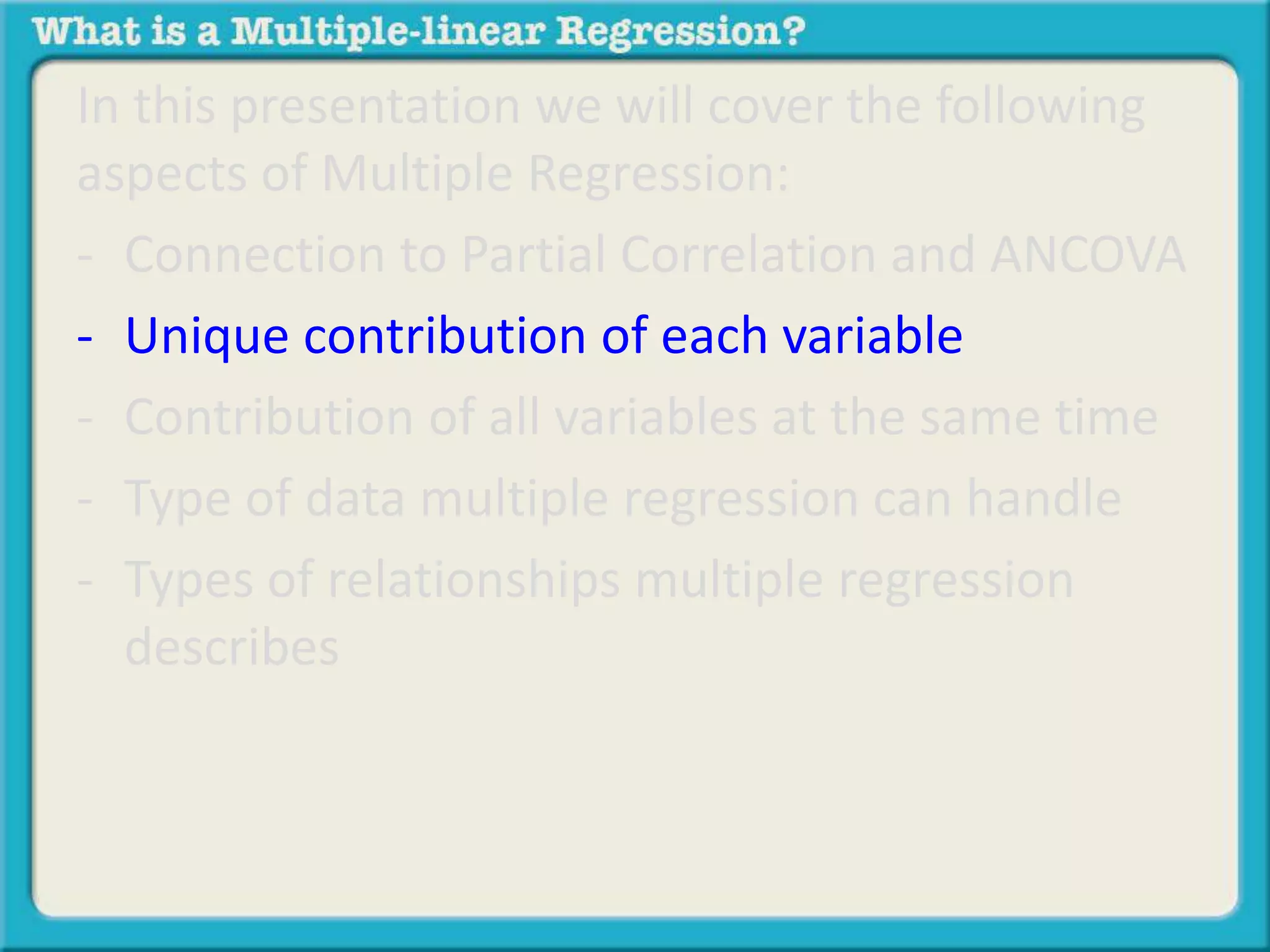
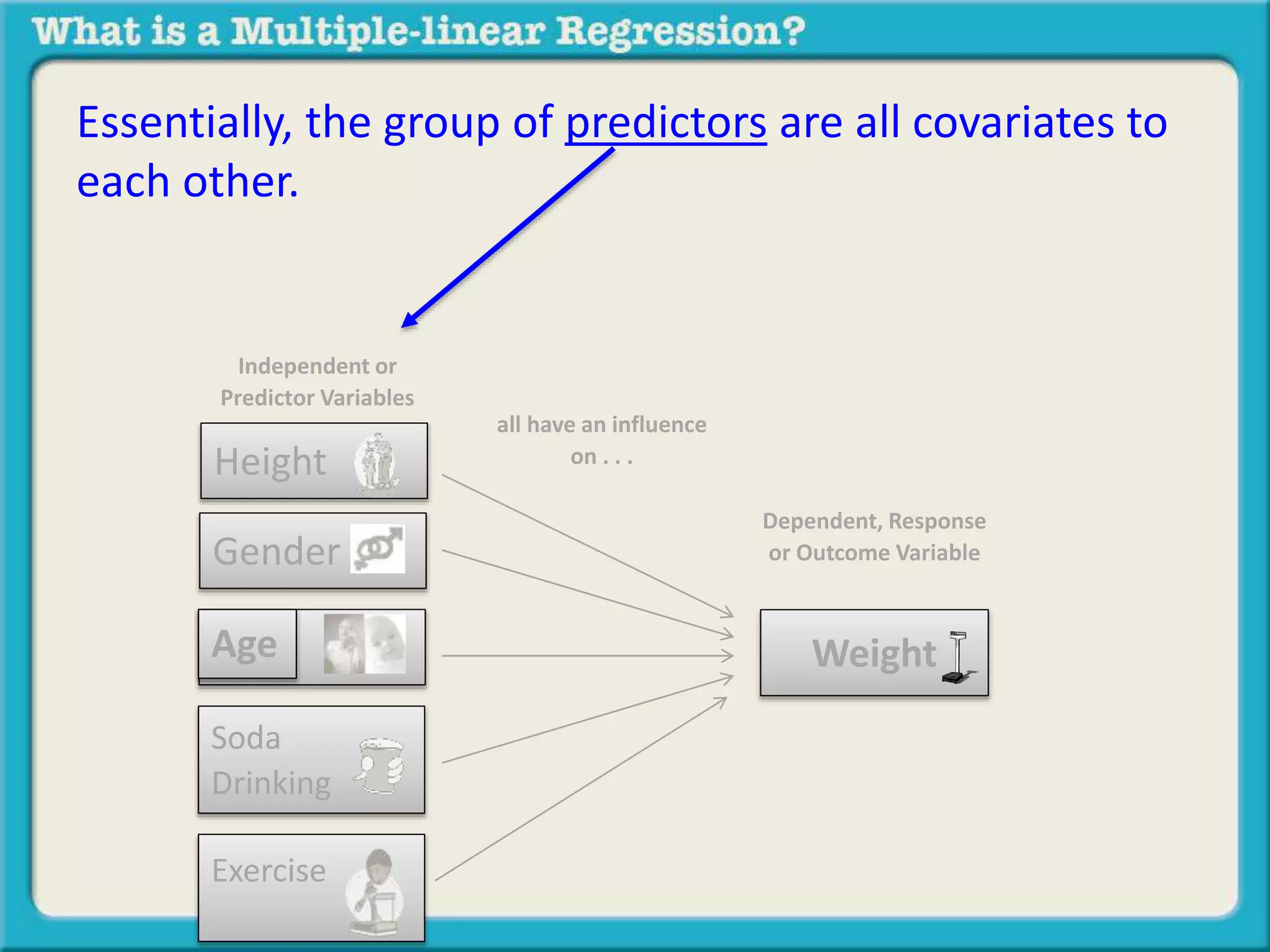
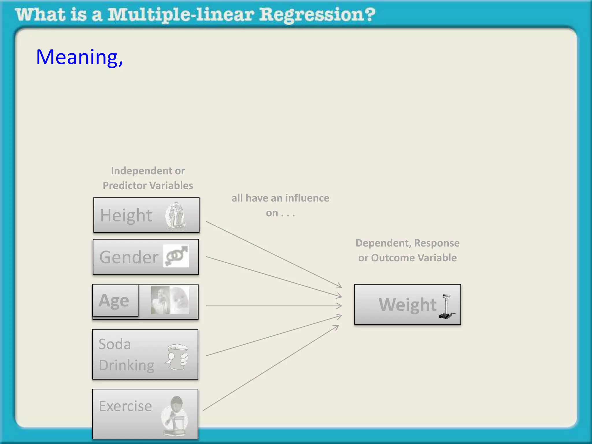
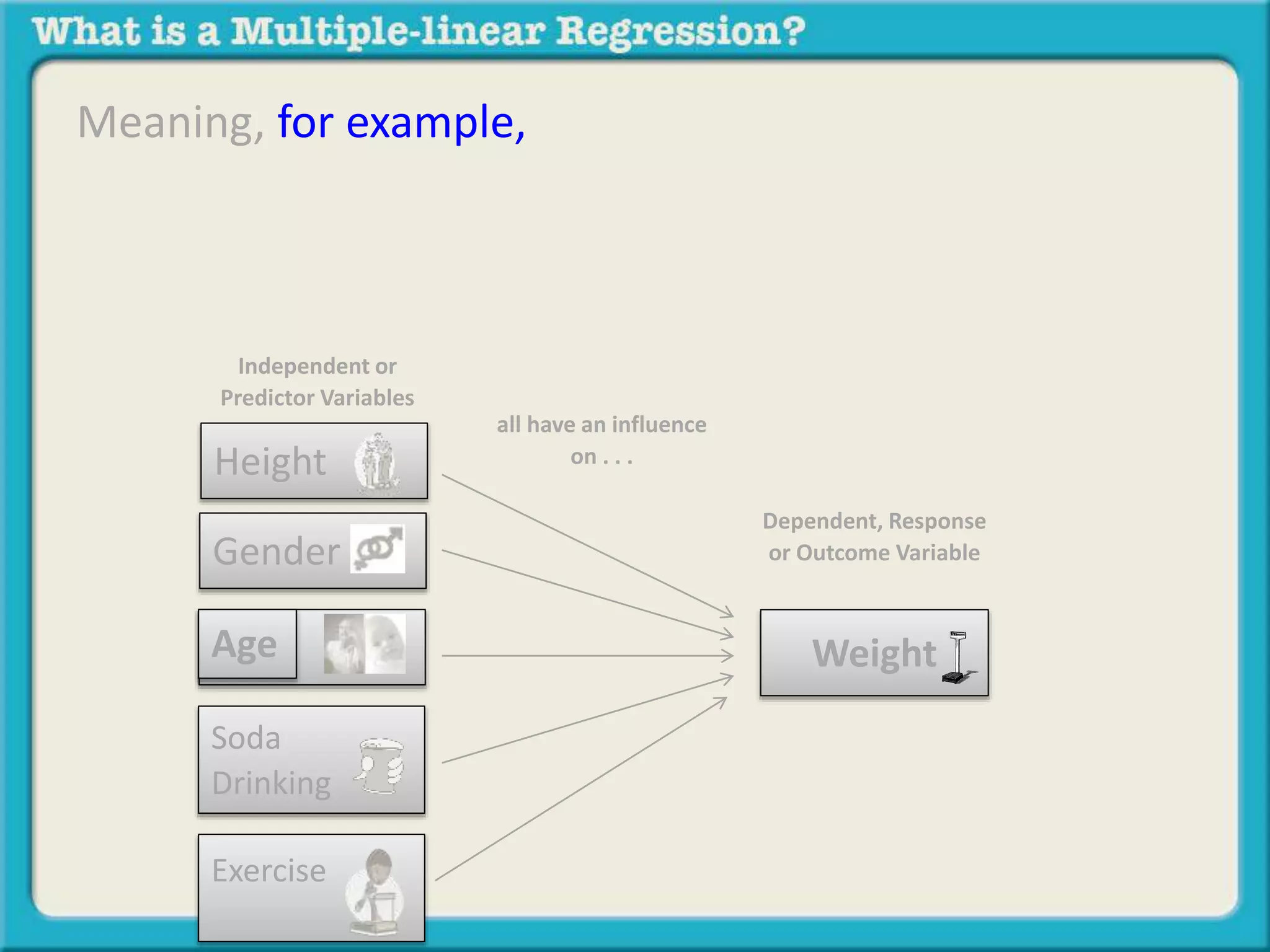
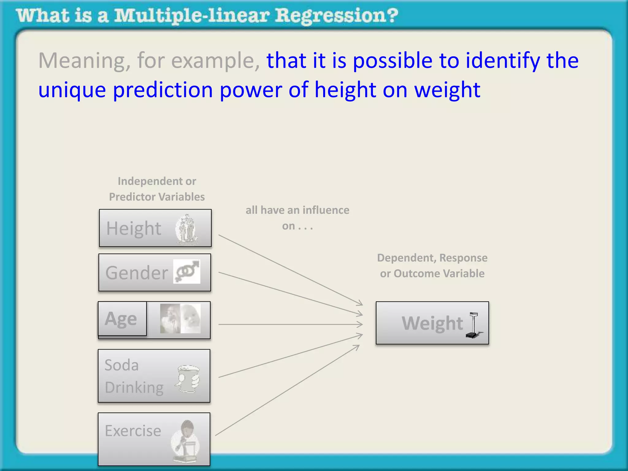
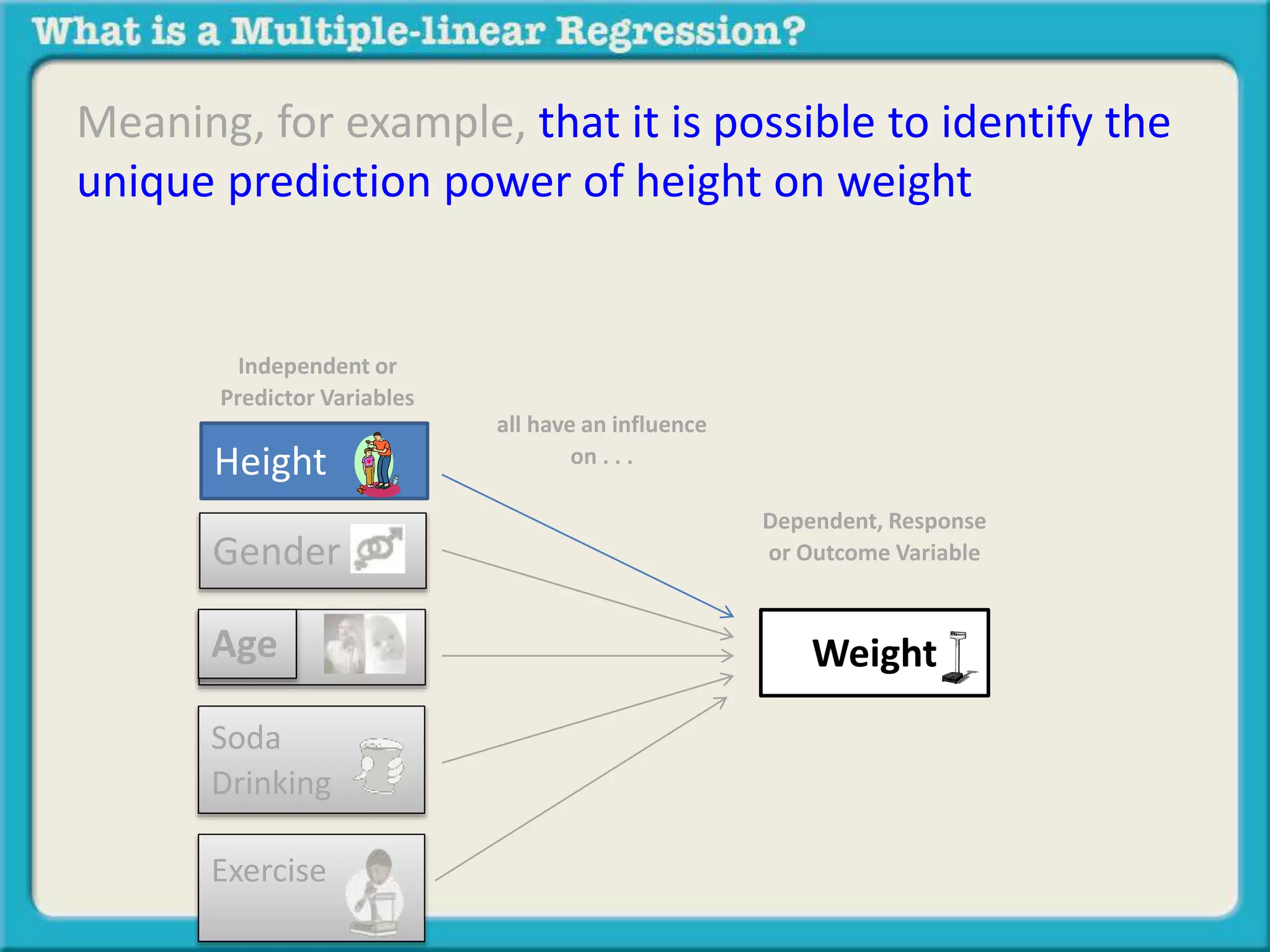
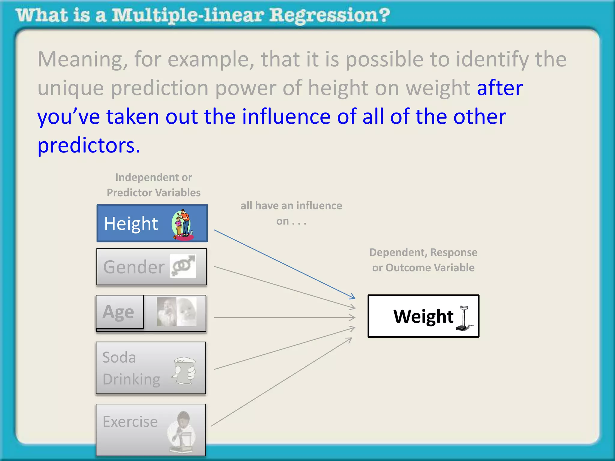
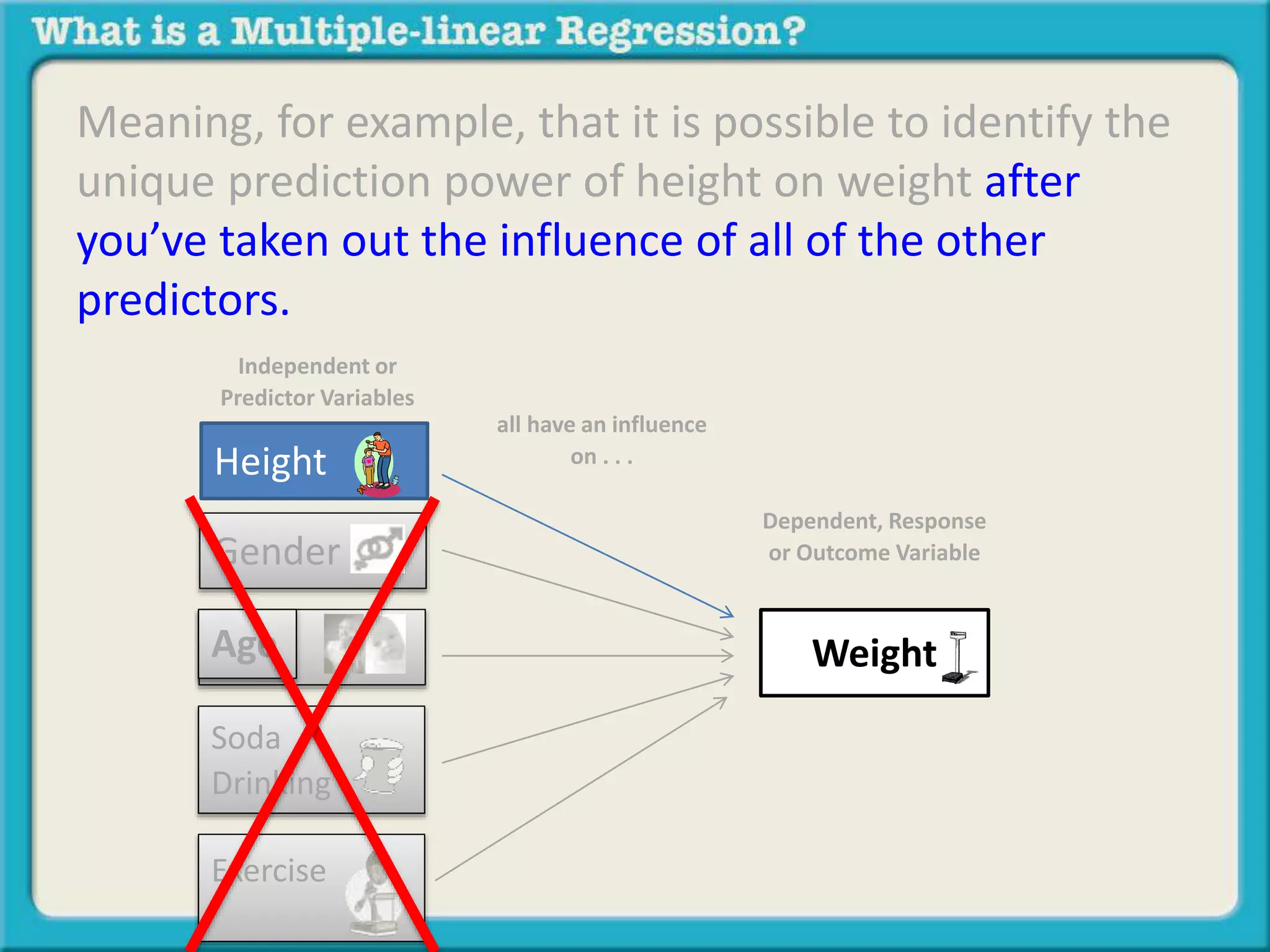
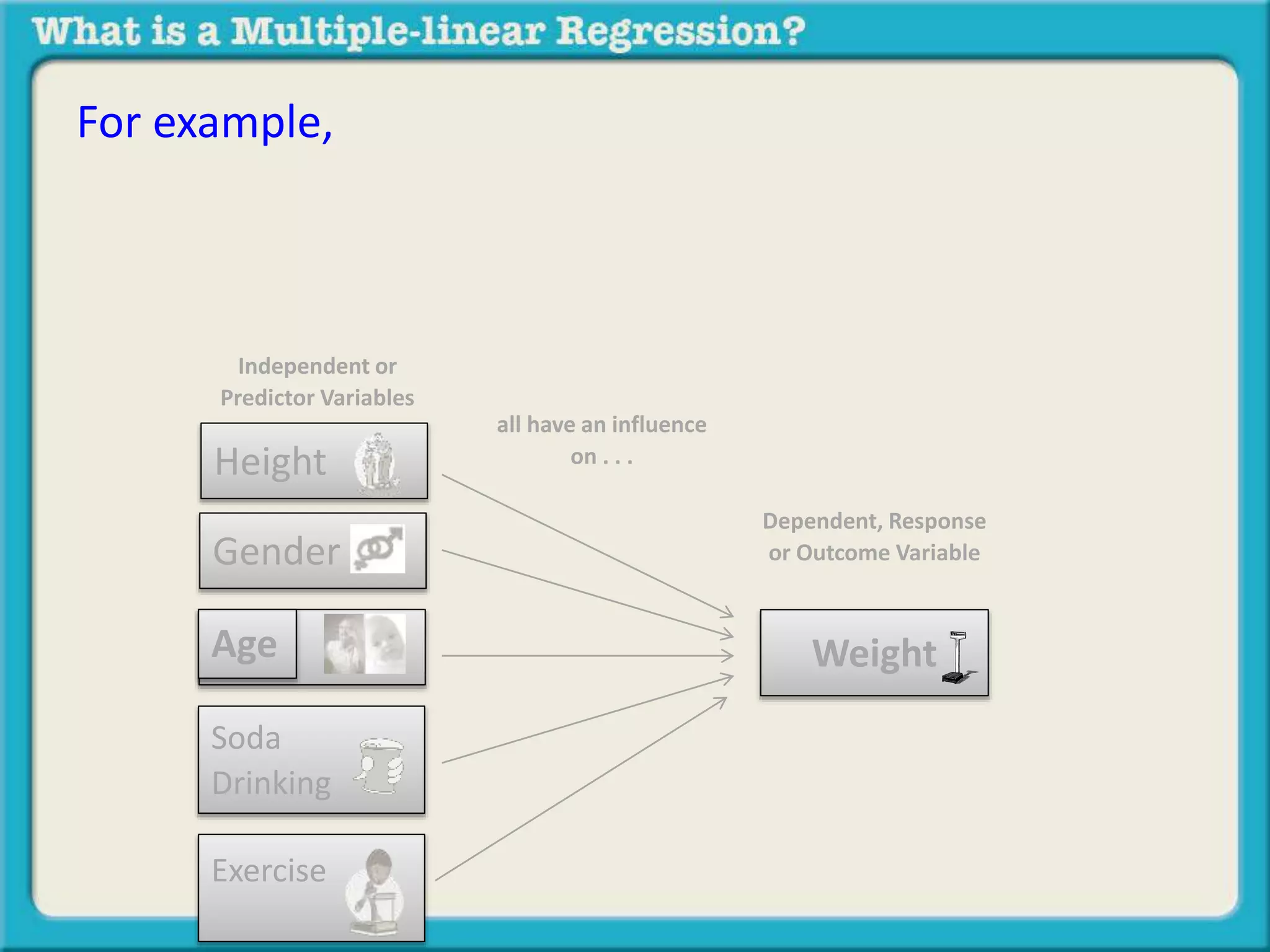
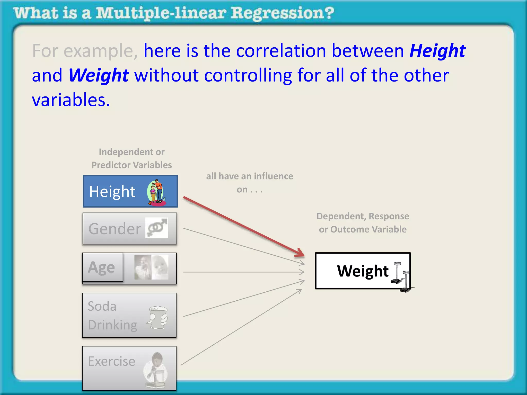
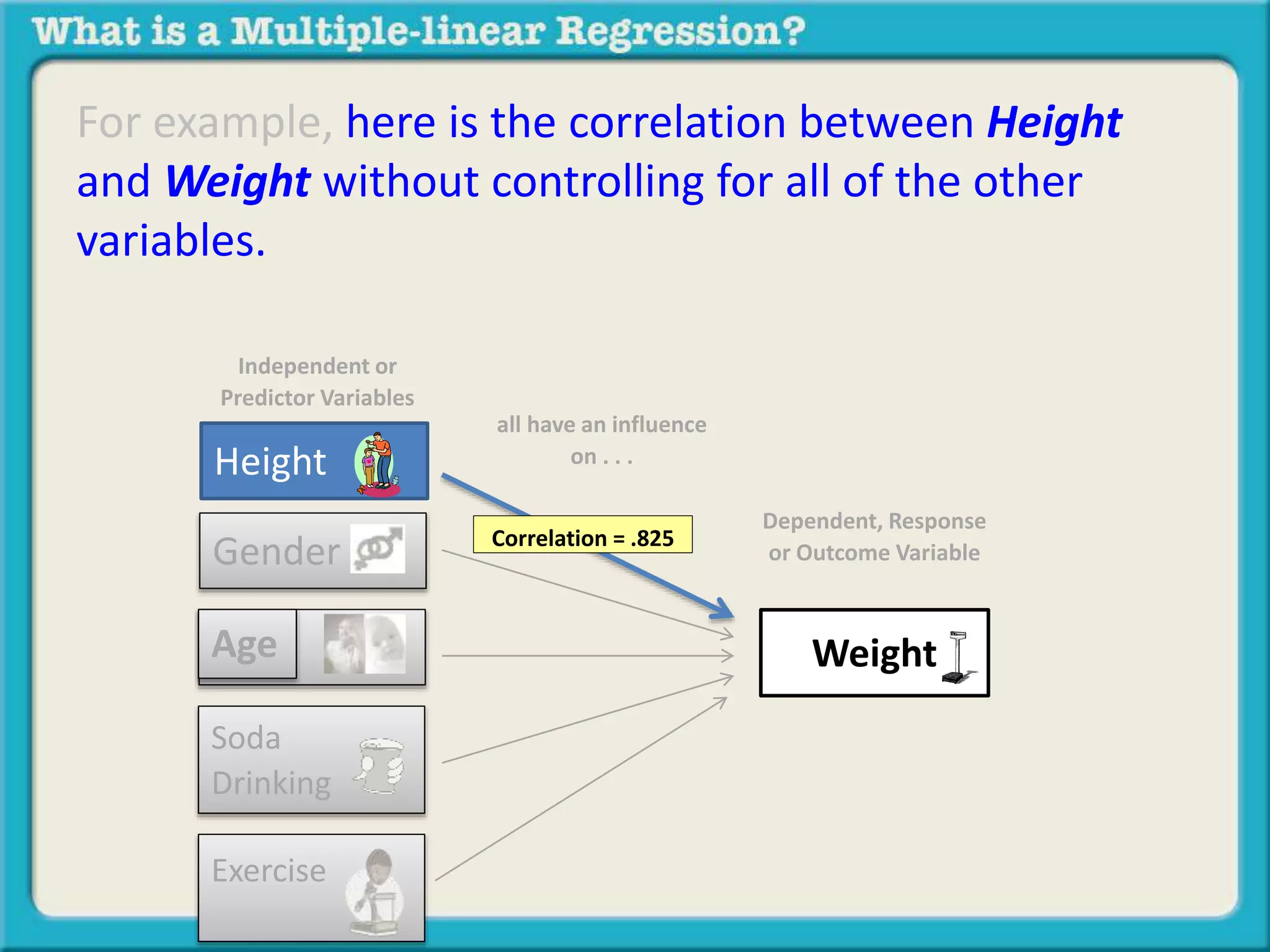
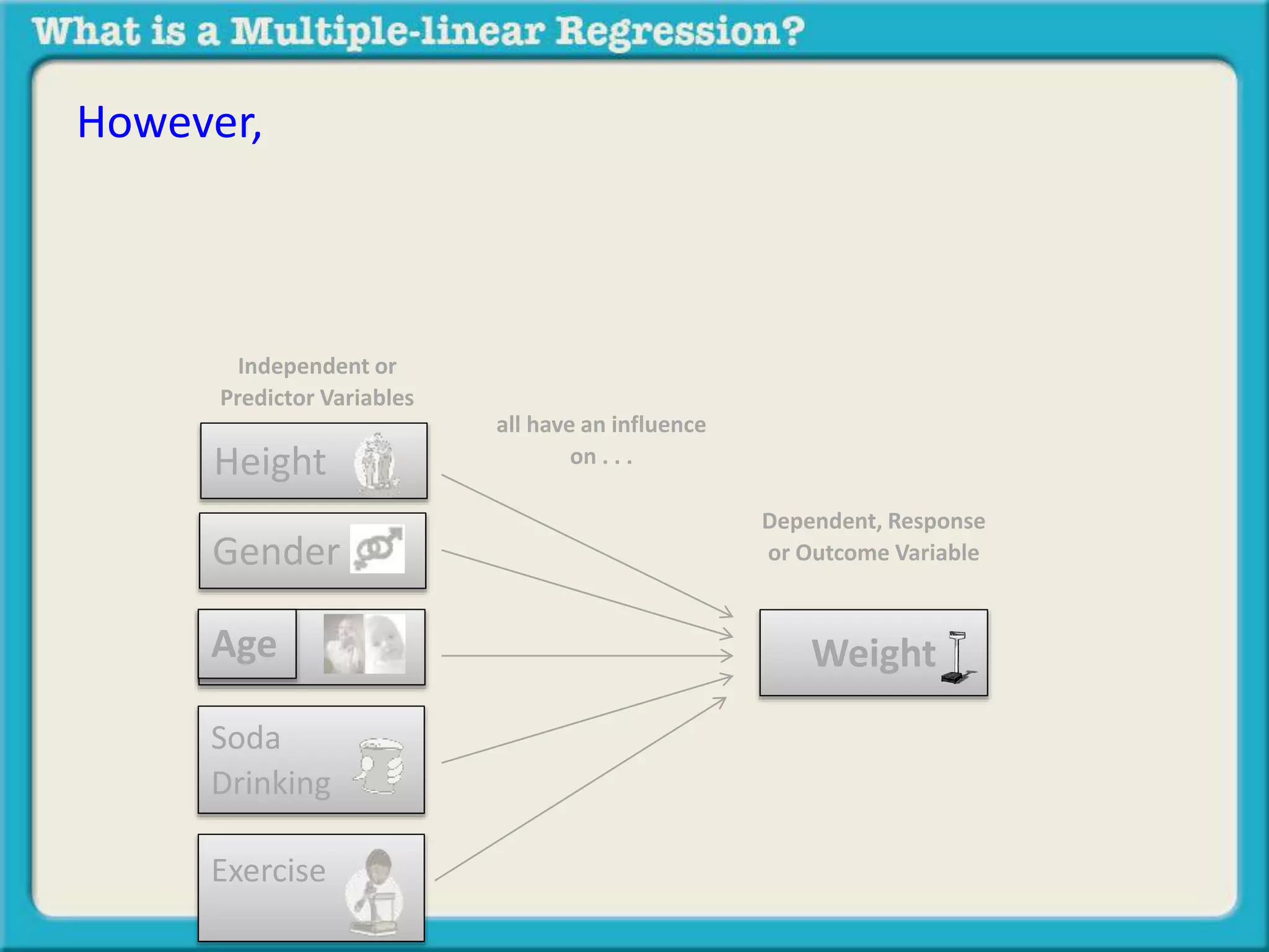
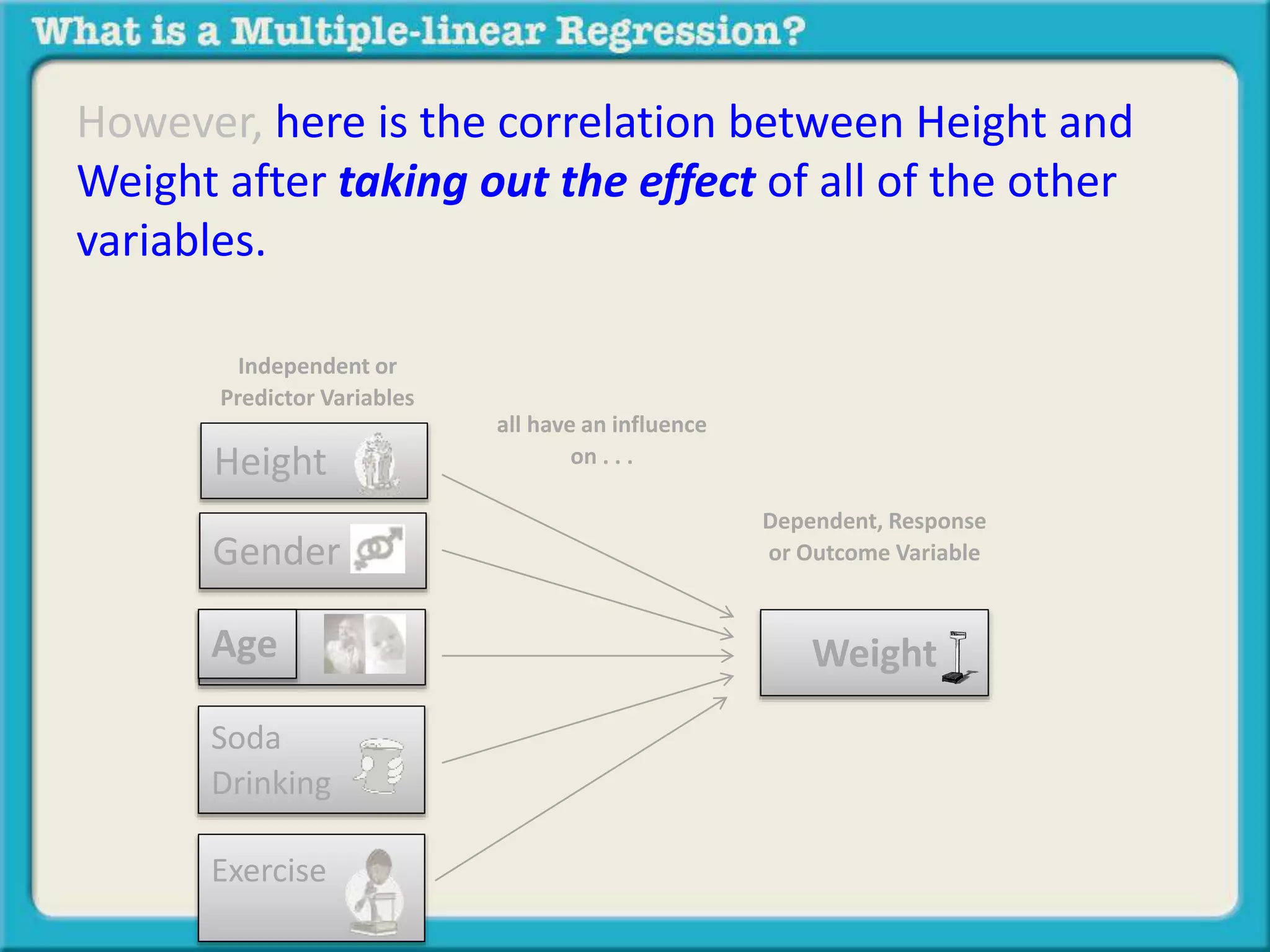
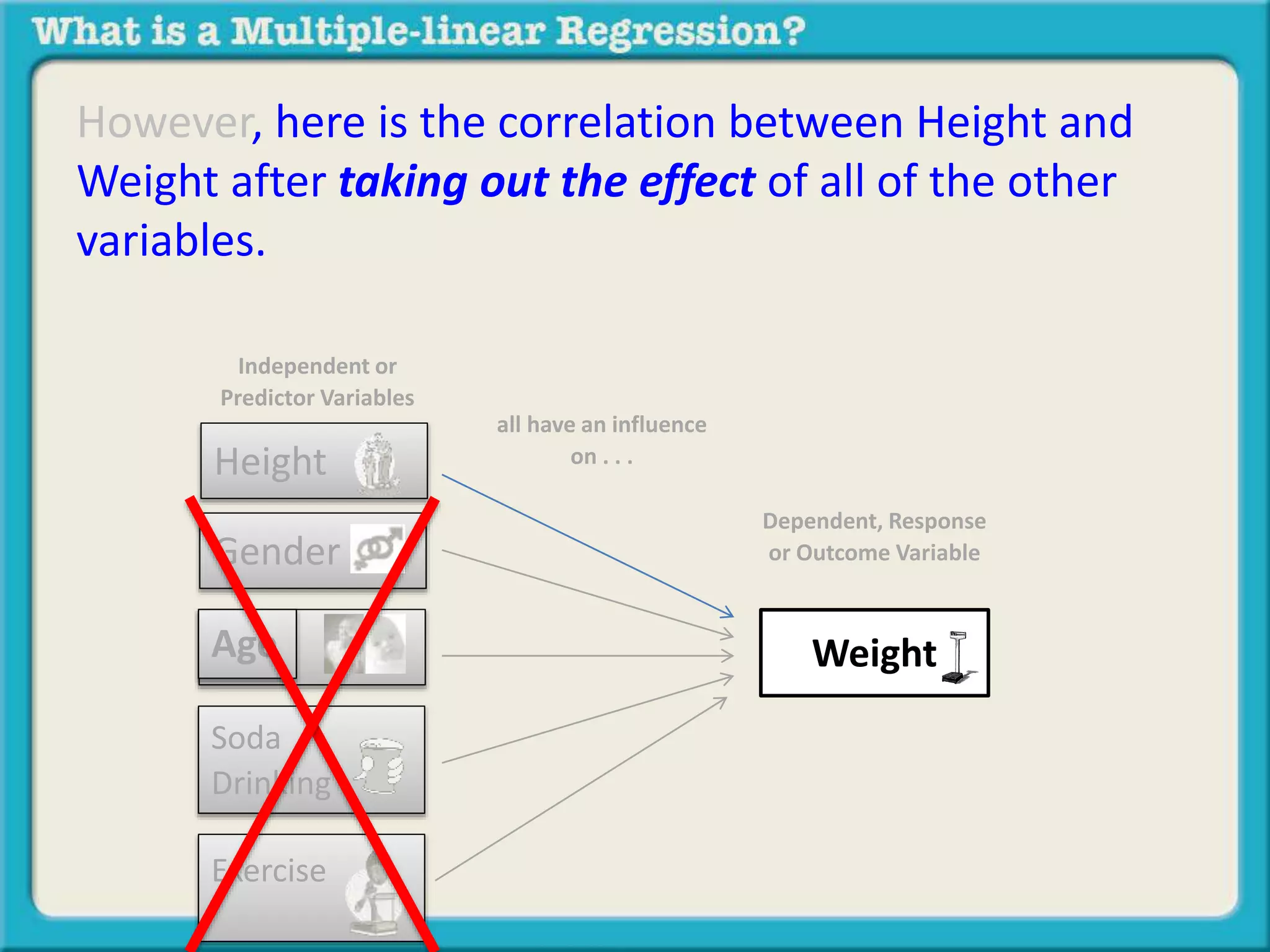
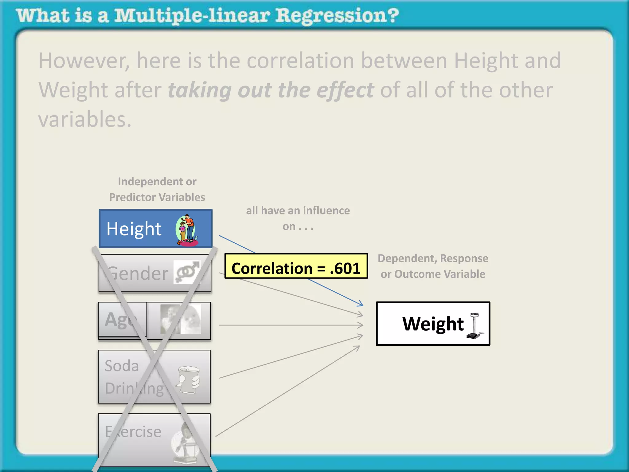
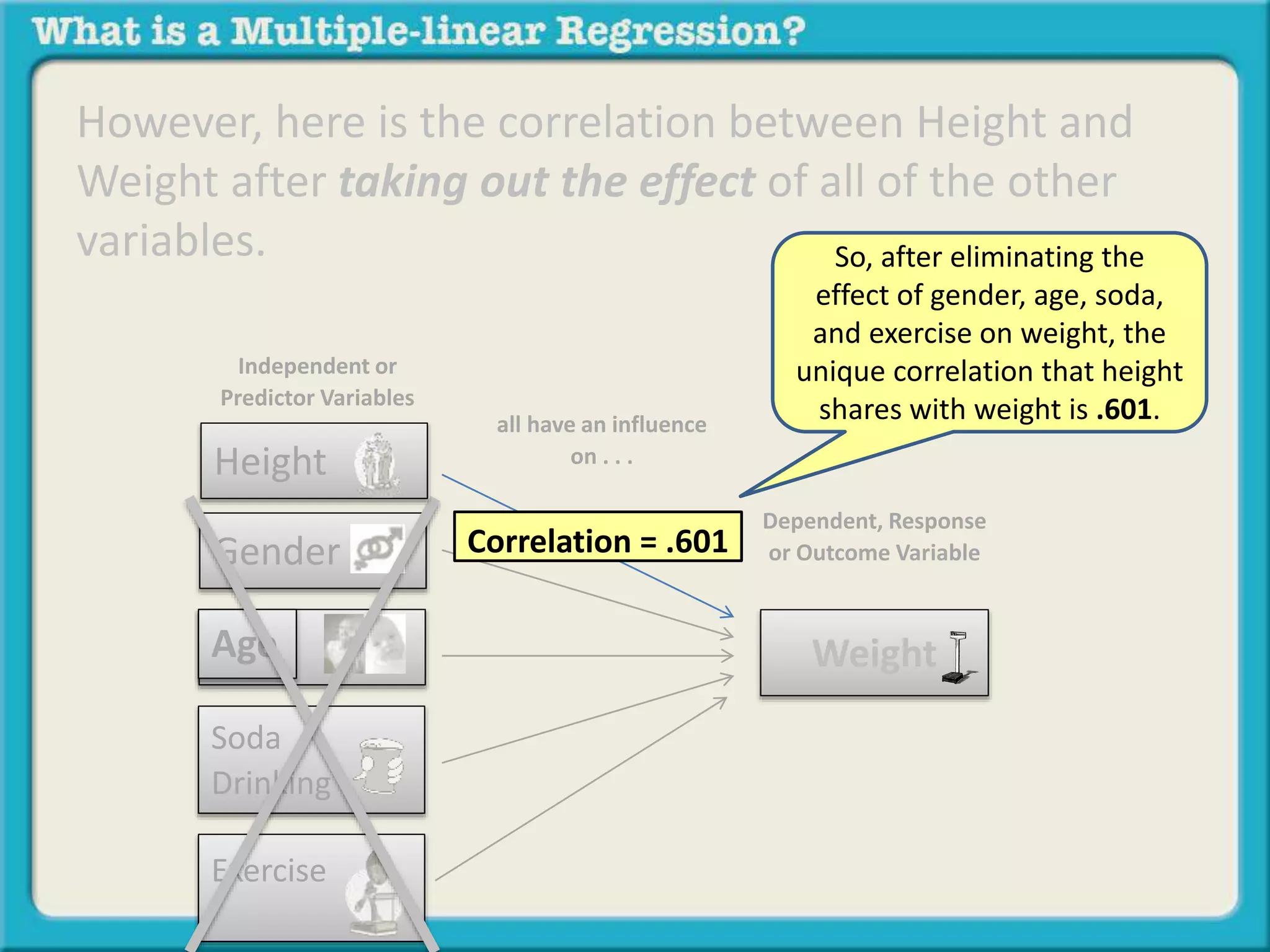
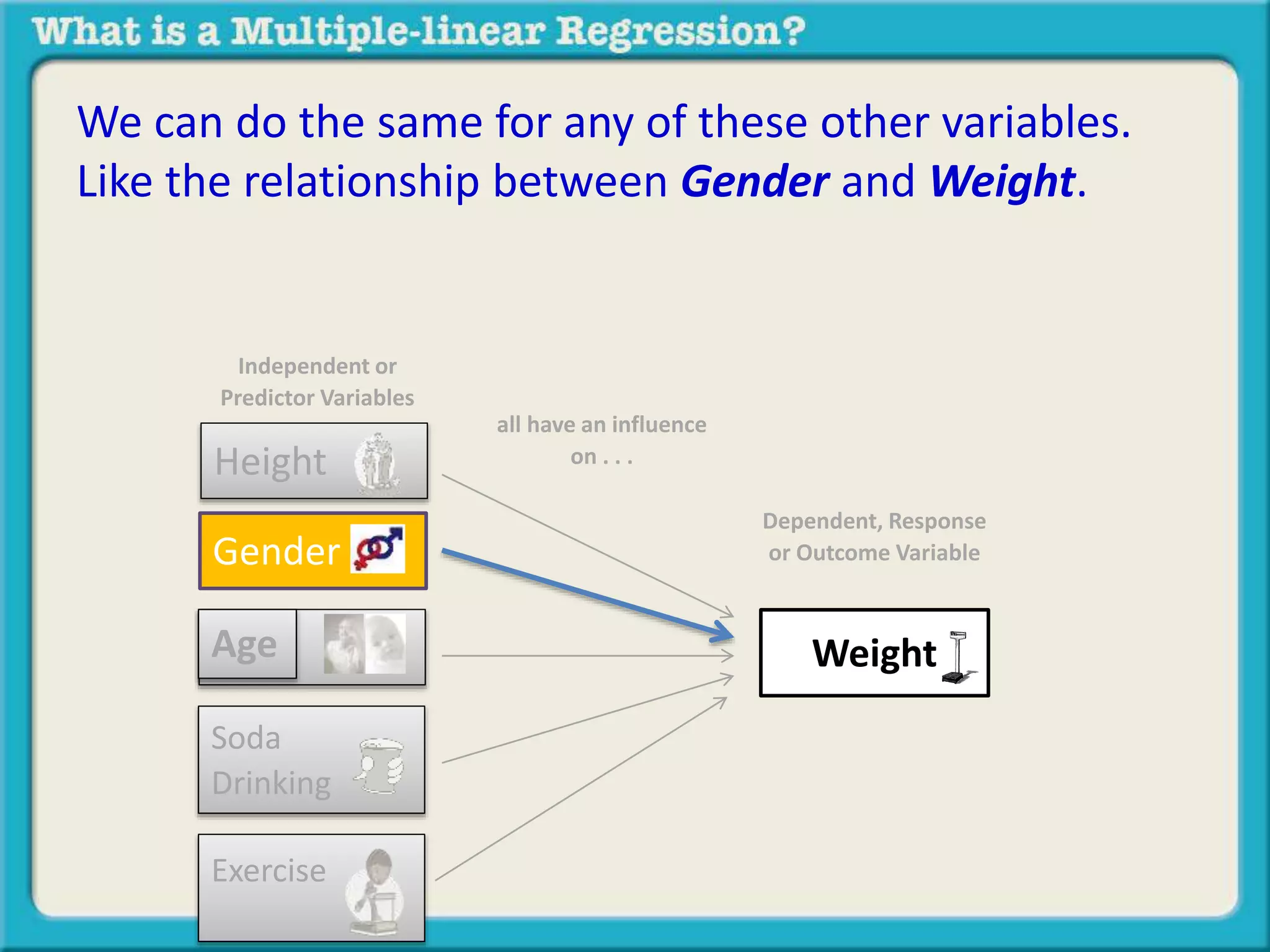
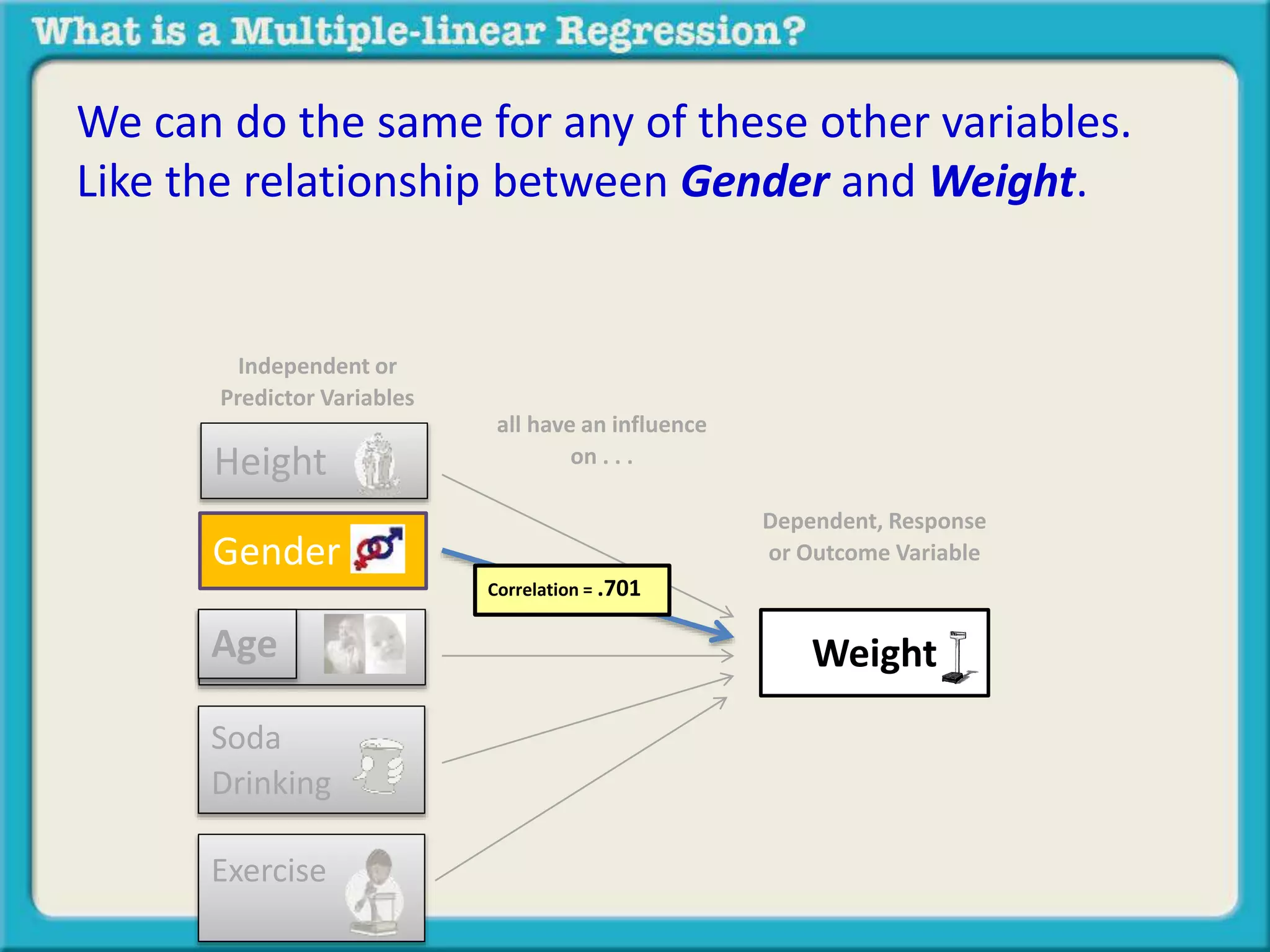
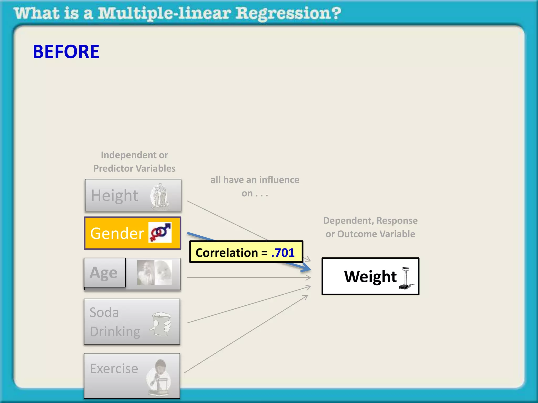
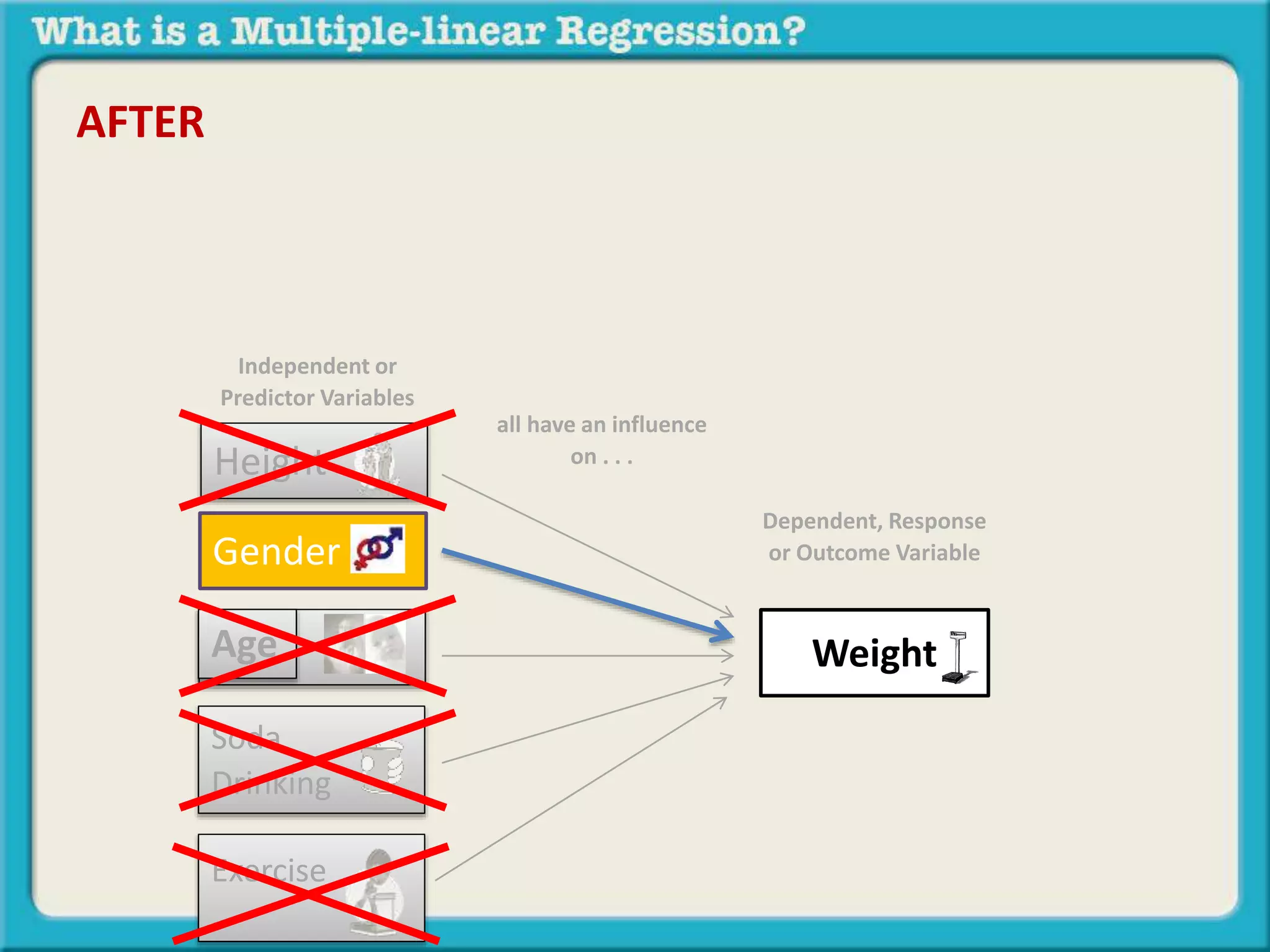
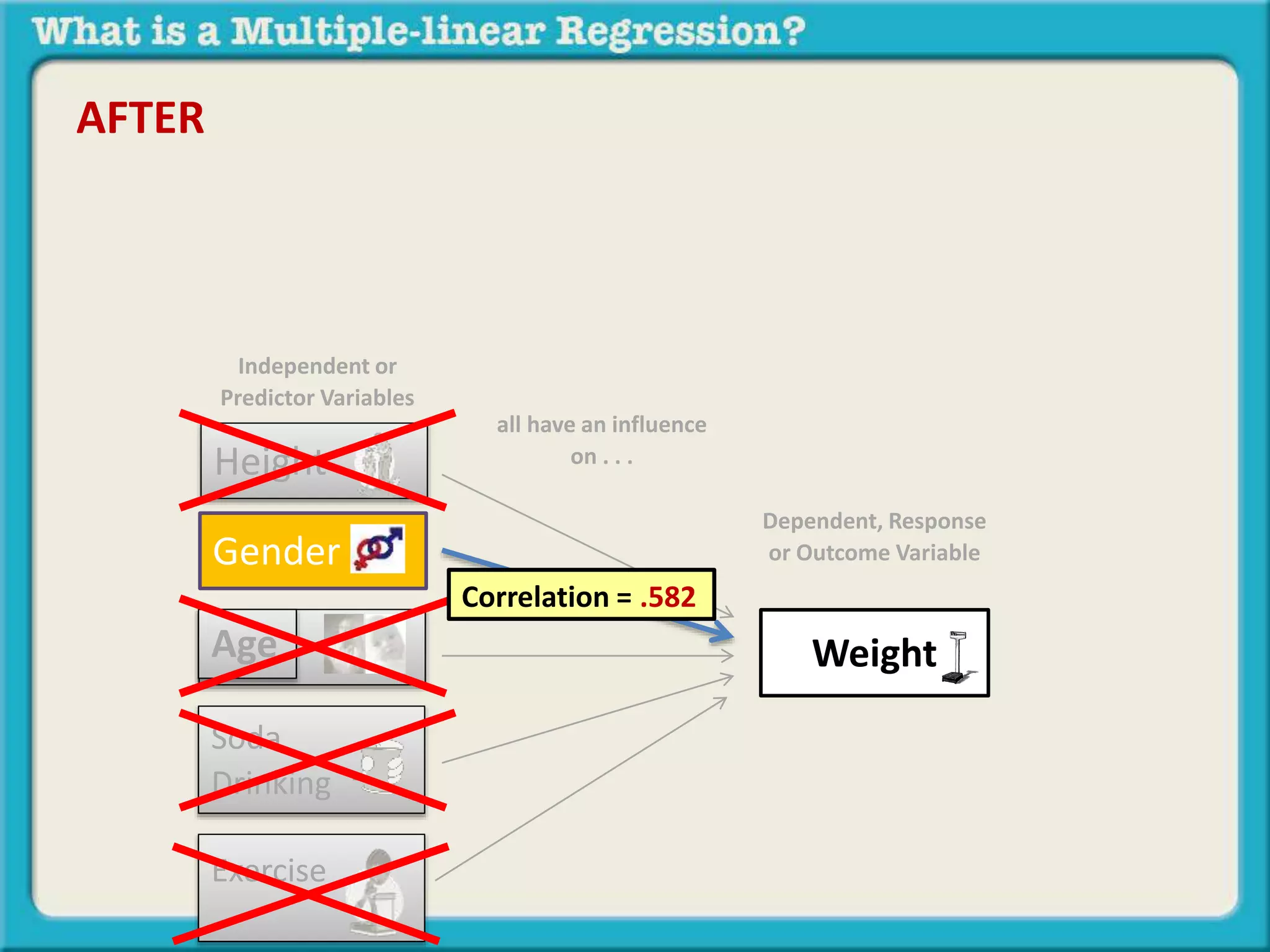
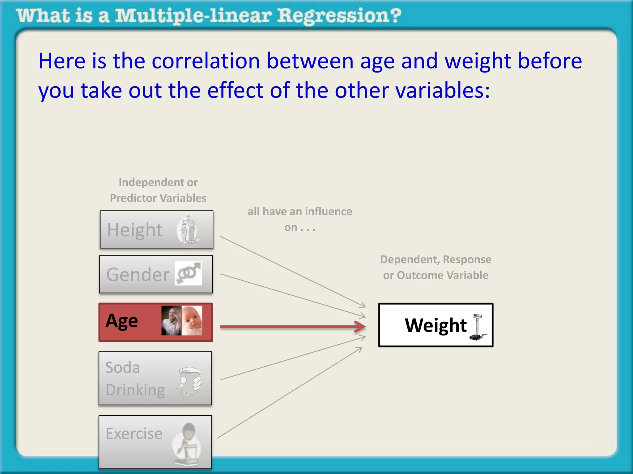
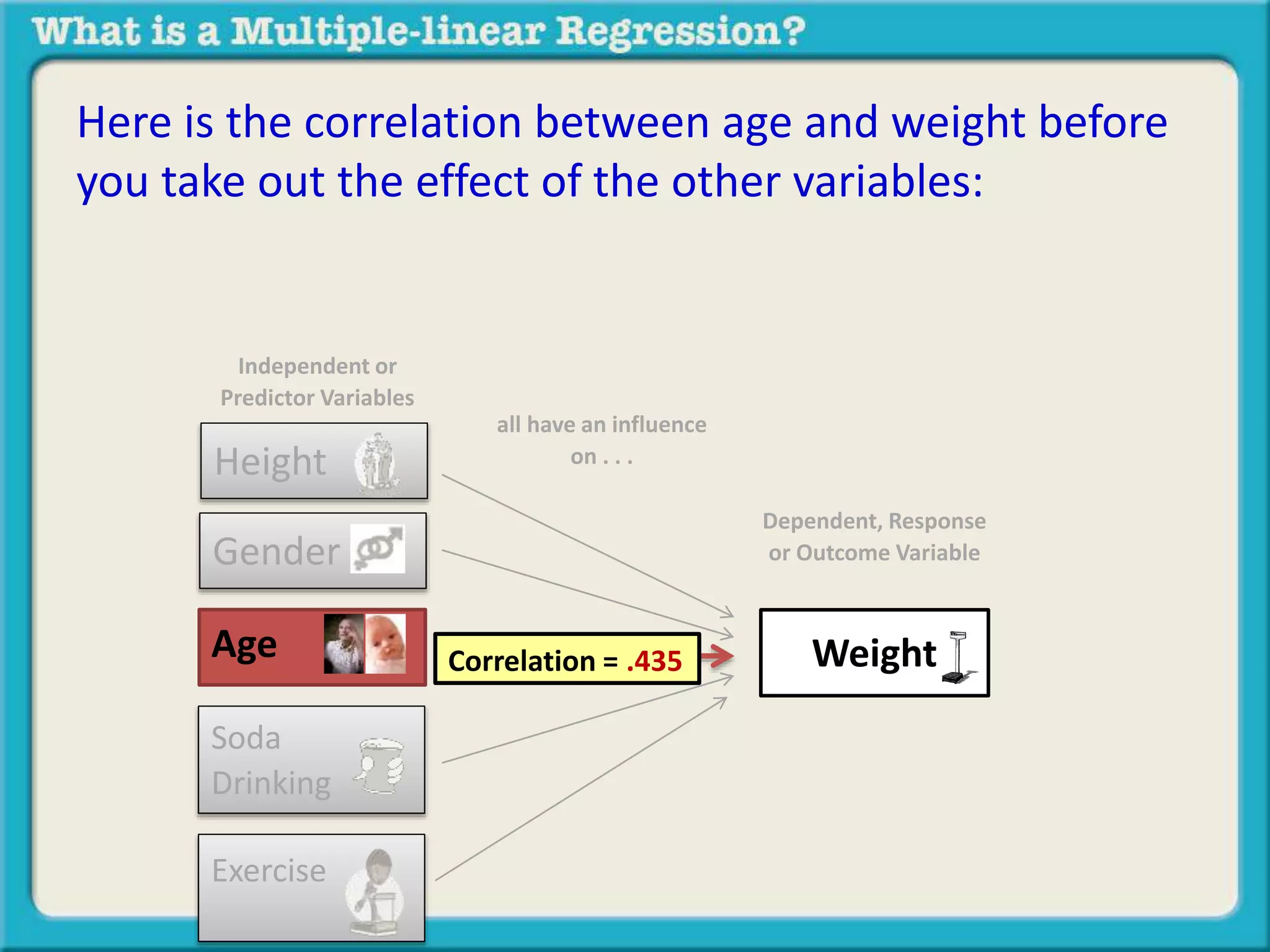
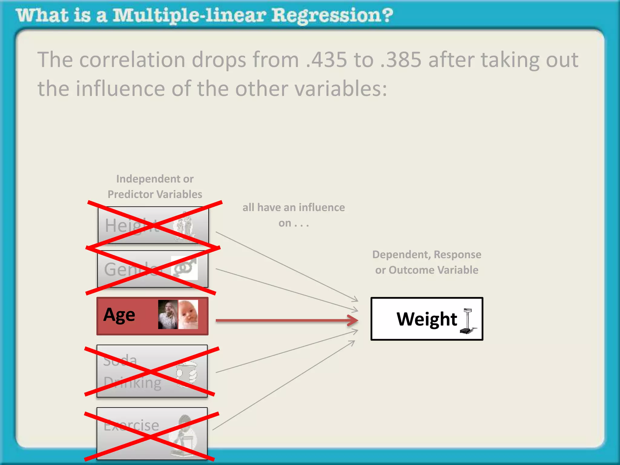
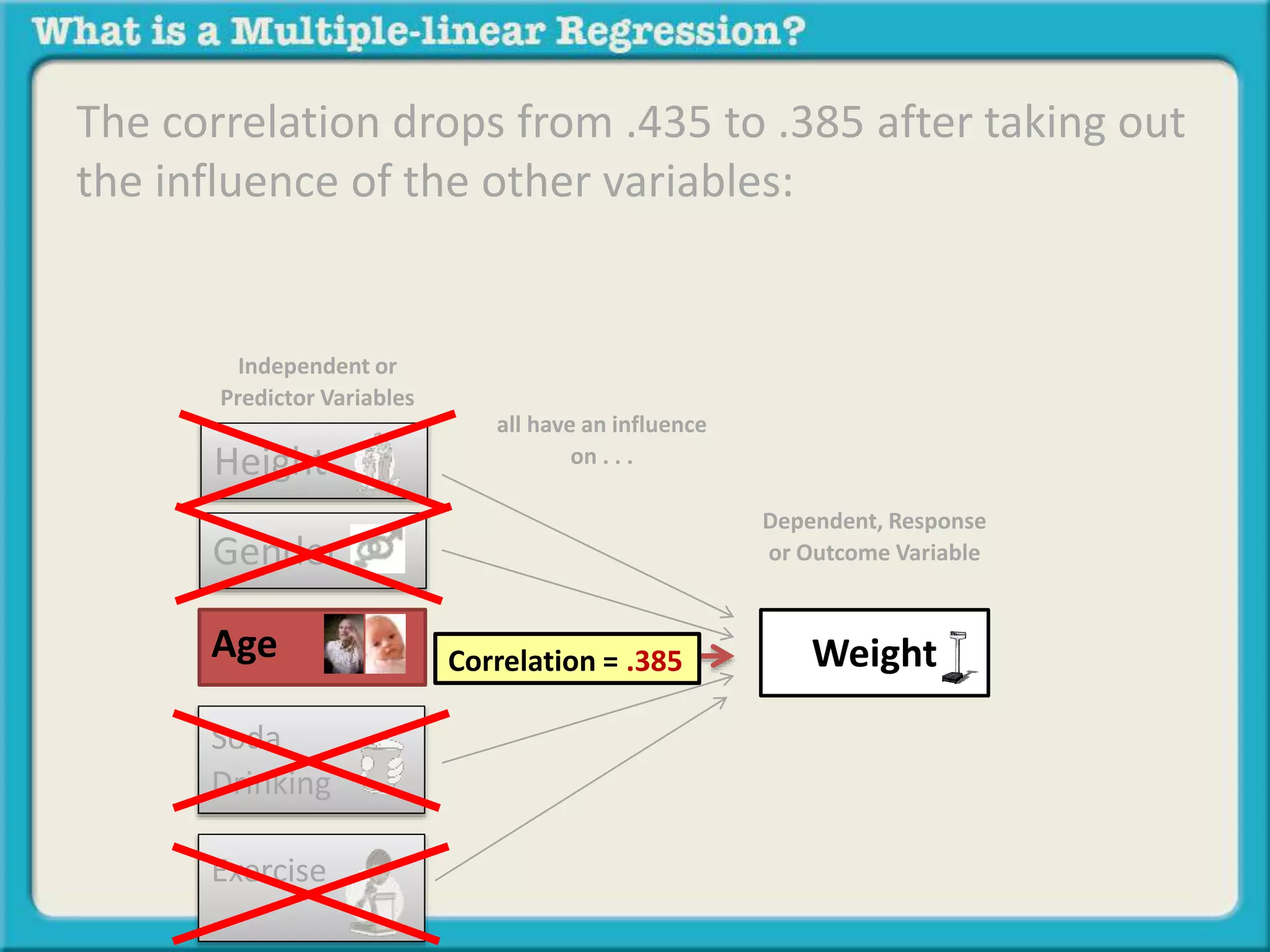
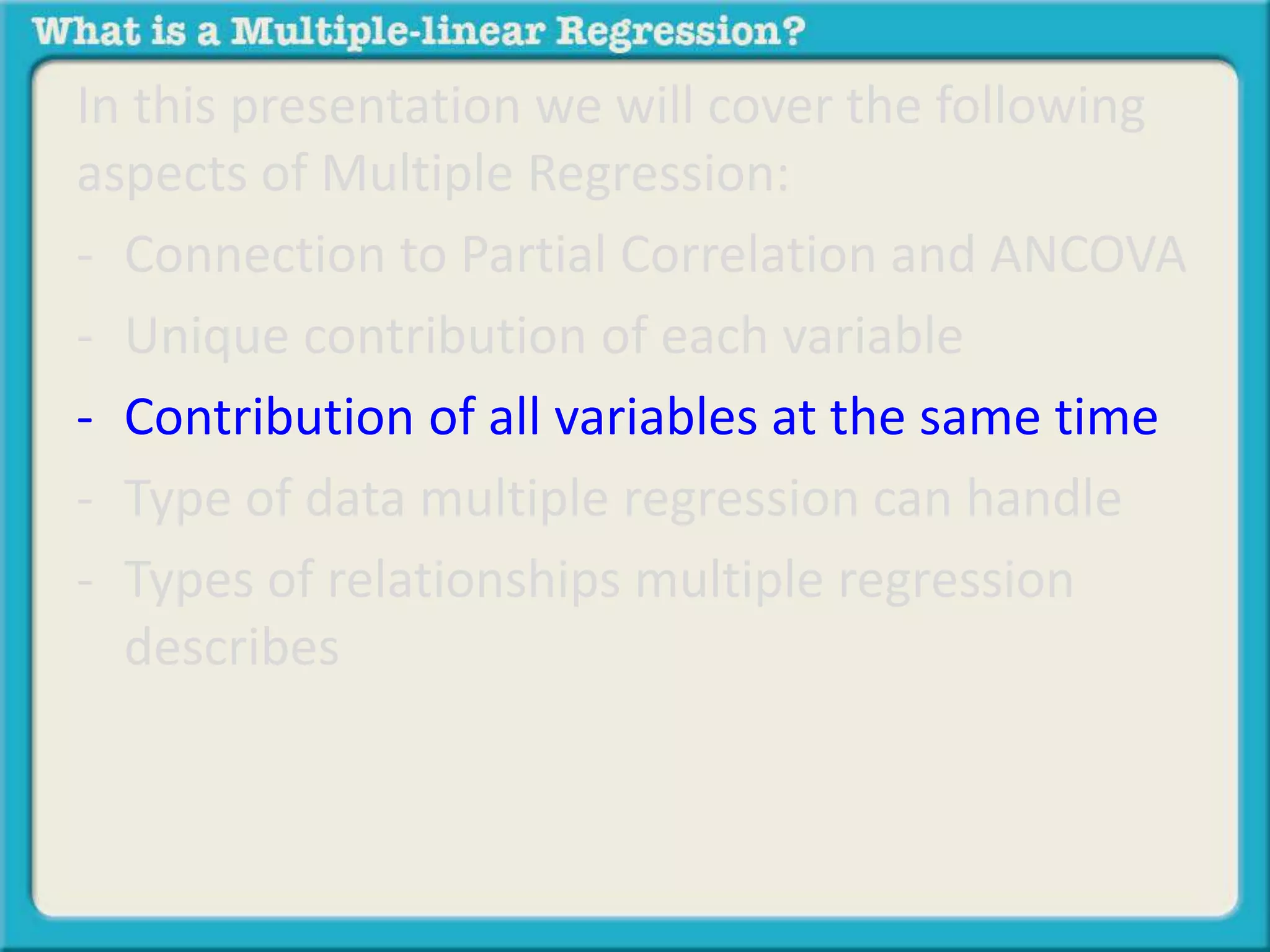
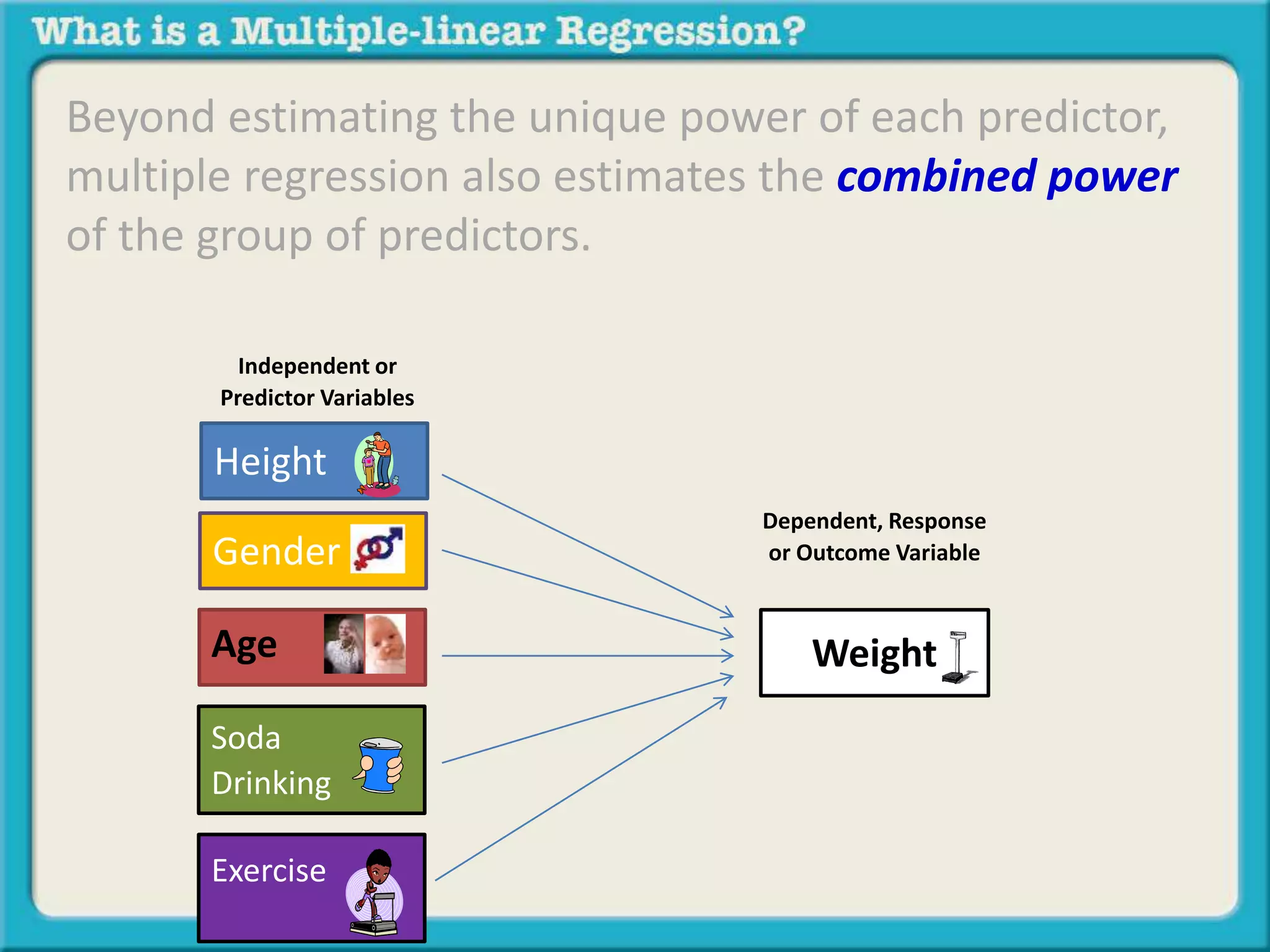
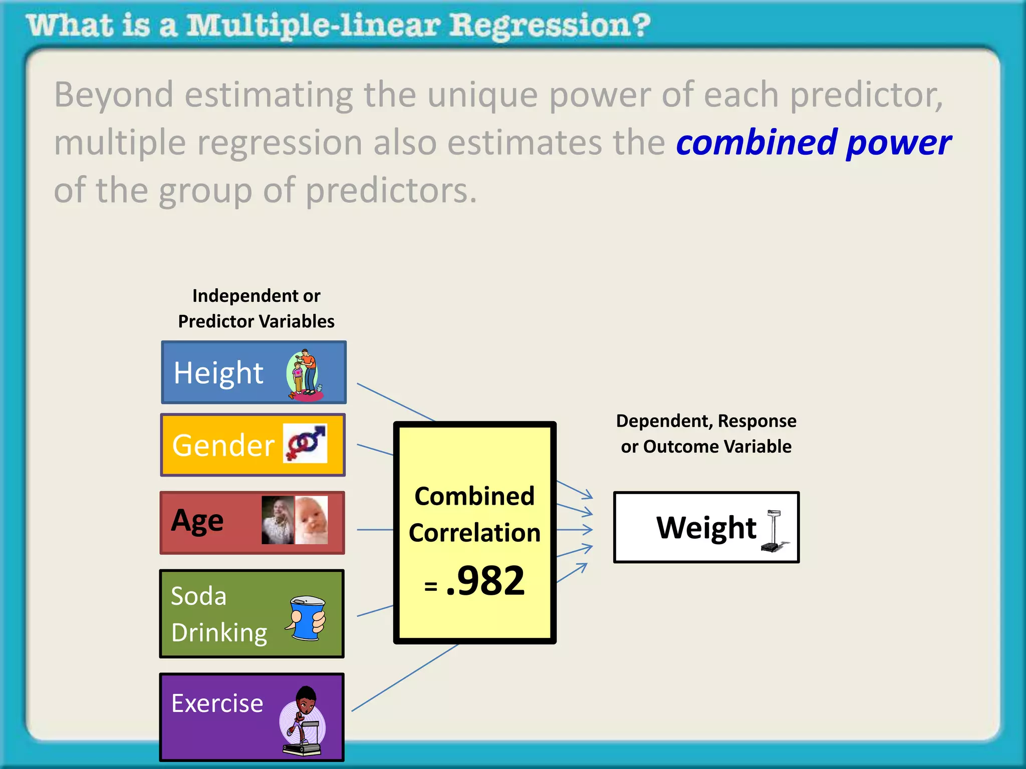
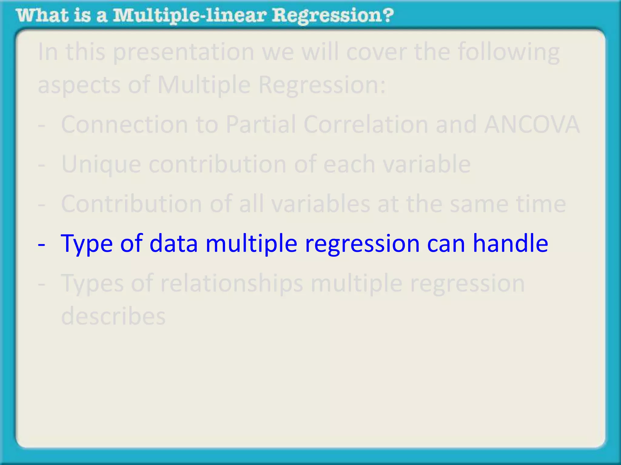
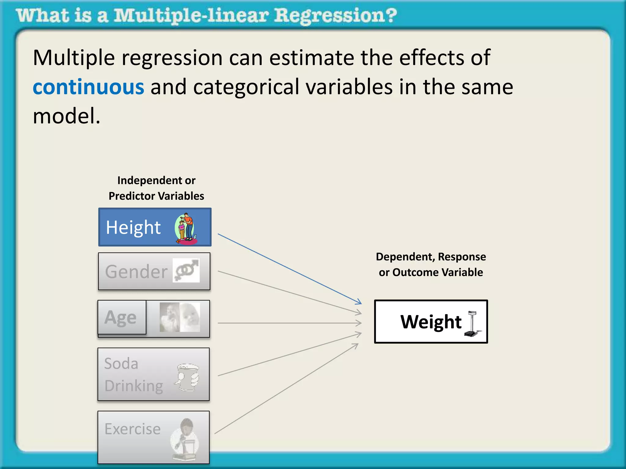
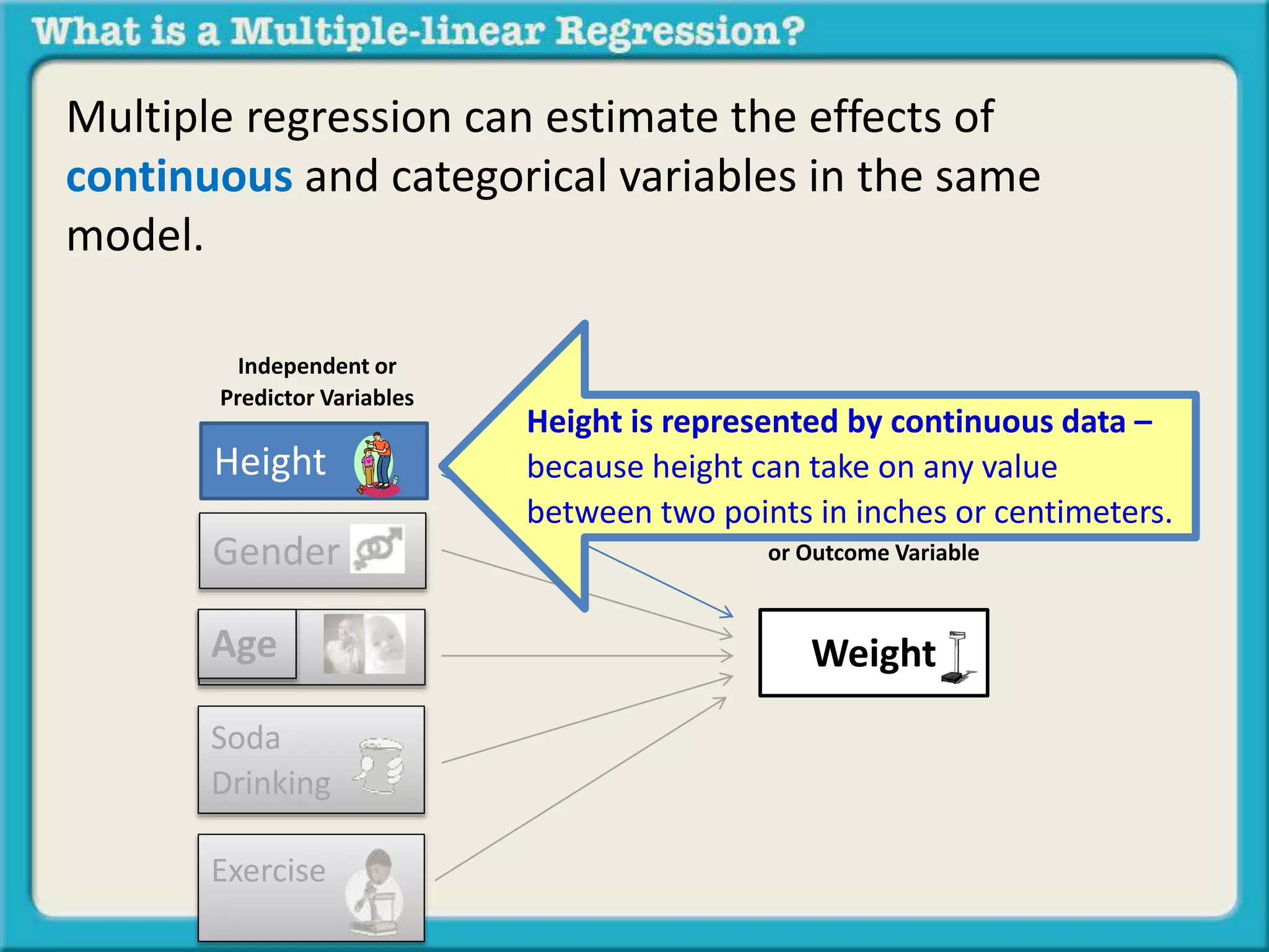
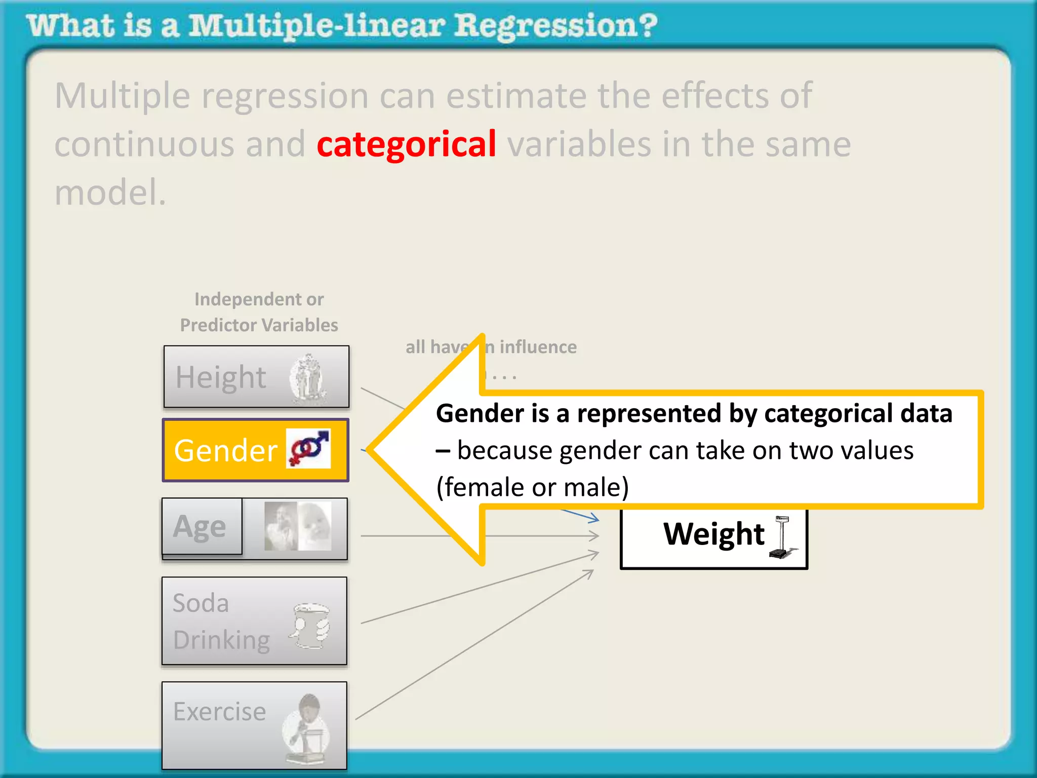
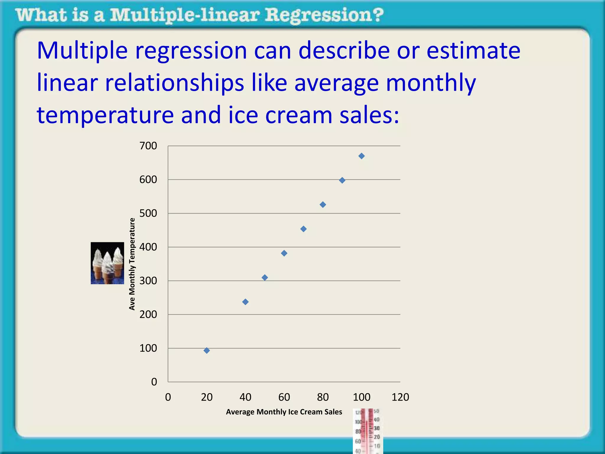
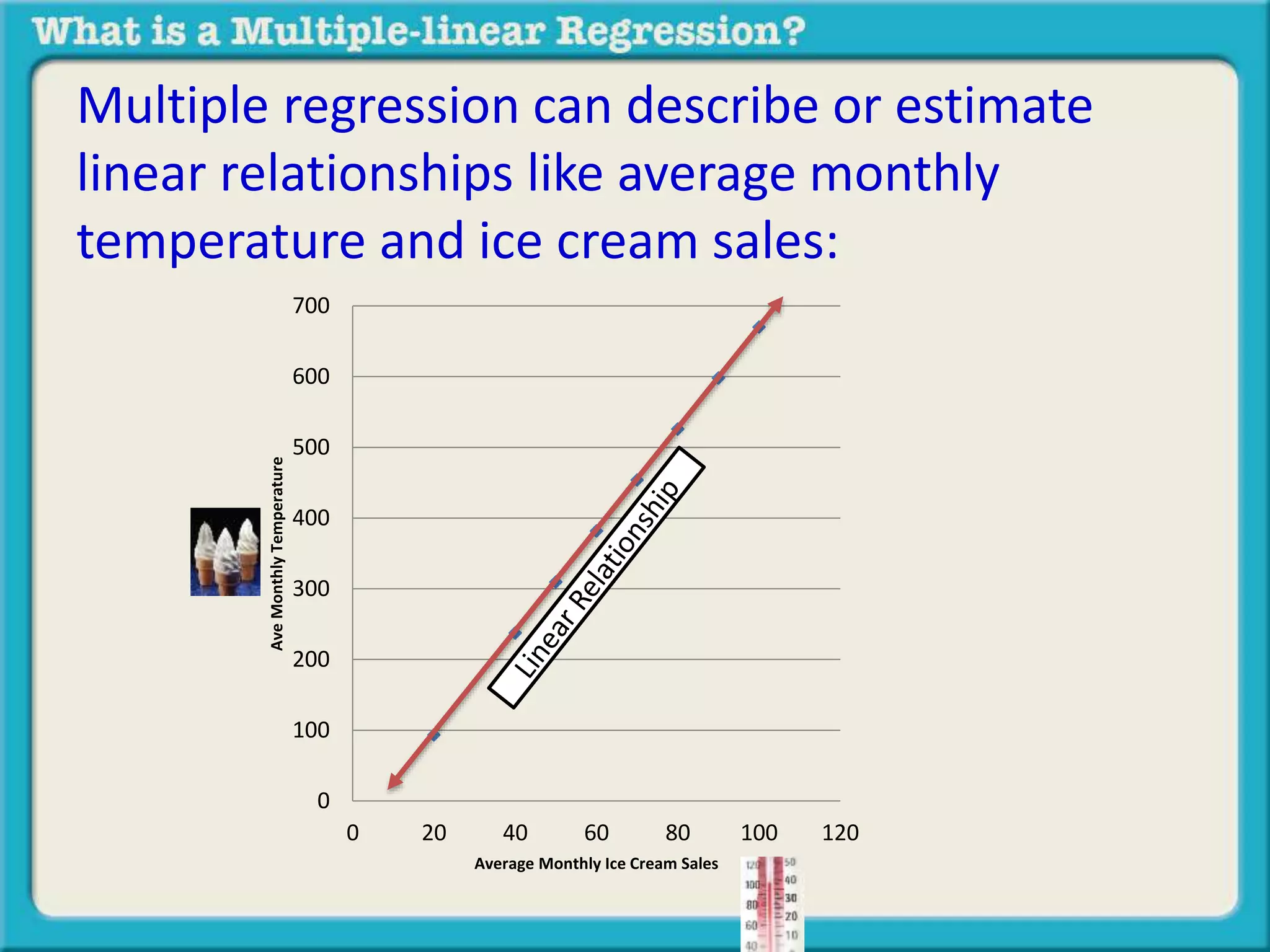
The document discusses multiple linear regression and partial correlation. It explains that multiple regression allows one to analyze the unique contribution of predictor variables to an outcome variable after accounting for the effects of other predictor variables. Partial correlation similarly examines the relationship between two variables while controlling for a third, but only considers two variables, whereas multiple regression examines the effects of multiple predictor variables simultaneously. Examples are given comparing the correlation between height and weight with and without controlling for other relevant variables like gender, age, exercise habits, etc.
Correlation & Regression Analysis using SPSSParag Shah
Concept of Correlation, Simple Linear Regression & Multiple Linear Regression and its analysis using SPSS. How it check the validity of assumptions in Regression
Multiple Regression and Logistic RegressionKaushik Rajan
1) Multiple Regression to predict Life Expectancy using independent variables Lifeexpectancymale, Lifeexpectancyfemale, Adultswhosmoke, Bingedrinkingadults, Healthyeatingadults and Physicallyactiveadults.
2) Binomial Logistic Regression to predict the Gender (0 - Male, 1 - Female) with the help of independent variables such as LifeExpectancy, Smokingadults, DrinkingAdults, Physicallyactiveadults and Healthyeatingadults.
Tools used:
> RStudio for Data pre-processing and exploratory data analysis
> SPSS for building the models
> LATEX for documentation
Introduces and explains the use of multiple linear regression, a multivariate correlational statistical technique. For more info, see the lecture page at http://goo.gl/CeBsv. See also the slides for the MLR II lecture http://www.slideshare.net/jtneill/multiple-linear-regression-ii
Simple Linear Regression: Step-By-StepDan Wellisch
This presentation was made to our meetup group found here.: https://www.meetup.com/Chicago-Technology-For-Value-Based-Healthcare-Meetup/ on 9/26/2017. Our group is focused on technology applied to healthcare in order to create better healthcare.
It is very difficult to distinguish the differences between ANOVA and regression. This is because both terms have more similarities than differences. It can be said that ANOVA and regression are the two sides of the same coin.
Overviews non-parametric and parametric approaches to (bivariate) linear correlation. See also: http://en.wikiversity.org/wiki/Survey_research_and_design_in_psychology/Lectures/Correlation
36030 Topic Discussion1Number of Pages 2 (Double Spaced).docxrhetttrevannion
36030 Topic: Discussion1
Number of Pages: 2 (Double Spaced)
Number of sources: 1
Writing Style: APA
Type of document: Essay
Academic Level:Master
Category: Psychology
Language Style: English (U.S.)
Order Instructions: Attached
I will upload the instruction
Reference/Article
Module 18: Correlational Research
Magnitude, Scatterplots, and Types of Relationships
Magnitude
Scatterplots
Positive Relationships
Negative Relationships
No Relationship
Curvilinear Relationships
Misinterpreting Correlations
The Assumptions of Causality and Directionality
The Third-Variable Problem
Restrictive Range
Curvilinear Relationships
Prediction and Correlation
Review of Key Terms
Module Exercises
Critical Thinking Check Answers
Module 19: Correlation Coefficients
The Pearson Product-Moment Correlation Coefficient: What It Is and What It Does
Calculating the Pearson Product-Moment Correlation
Interpreting the Pearson Product-Moment Correlation
Alternative Correlation Coefficients
Review of Key Terms
Module Exercises
Critical Thinking Check Answers
Module 20: Advanced Correlational Techniques: Regression Analysis
Regression Lines
Calculating the Slope and y-intercept
Prediction and Regression
Multiple Regression Analysis
Review of Key Terms
Module Exercises
Critical Thinking Check Answers
Chapter 9 Summary and Review
Chapter 9 Statistical Software Resources
In this chapter, we discuss correlational research methods and correlational statistics. As a research method, correlational designs allow us to describe the relationship between two measured variables. A correlation coefficient aids us by assigning a numerical value to the observed relationship. We begin with a discussion of how to conduct correlational research, the magnitude and the direction of correlations, and graphical representations of correlations. We then turn to special considerations when interpreting correlations, how to use correlations for predictive purposes, and how to calculate correlation coefficients. Lastly, we will discuss an advanced correlational technique, regression analysis.
MODULE 18
Correlational Research
Learning Objectives
•Describe the difference between strong, moderate, and weak correlation coefficients.
•Draw and interpret scatterplots.
•Explain negative, positive, curvilinear, and no relationship between variables.
•Explain how assuming causality and directionality, the third-variable problem, restrictive ranges, and curvilinear relationships can be problematic when interpreting correlation coefficients.
•Explain how correlations allow us to make predictions.
When conducting correlational studies, researchers determine whether two naturally occurring variables (for example, height and weight, or smoking and cancer) are related to each other. Such studies assess whether the variables are “co-related” in some way—do people who are taller tend to weigh more, or do those who smoke tend to have a higher incidence of cancer? As we saw in Chapter 1, the correlationa.
36033 Topic Happiness Data setNumber of Pages 2 (Double Spac.docxrhetttrevannion
36033 Topic: Happiness Data set
Number of Pages: 2 (Double Spaced)
Number of sources: 1
Writing Style: APA
Type of document: Essay
Academic Level:Master
Category: Psychology
Language Style: English (U.S.)
Order Instructions: Attached
I will upload the instructions
Reference/Article
Module 18: Correlational Research
Magnitude, Scatterplots, and Types of Relationships
Magnitude
Scatterplots
Positive Relationships
Negative Relationships
No Relationship
Curvilinear Relationships
Misinterpreting Correlations
The Assumptions of Causality and Directionality
The Third-Variable Problem
Restrictive Range
Curvilinear Relationships
Prediction and Correlation
Review of Key Terms
Module Exercises
Critical Thinking Check Answers
Module 19: Correlation Coefficients
The Pearson Product-Moment Correlation Coefficient: What It Is and What It Does
Calculating the Pearson Product-Moment Correlation
Interpreting the Pearson Product-Moment Correlation
Alternative Correlation Coefficients
Review of Key Terms
Module Exercises
Critical Thinking Check Answers
Module 20: Advanced Correlational Techniques: Regression Analysis
Regression Lines
Calculating the Slope and y-intercept
Prediction and Regression
Multiple Regression Analysis
Review of Key Terms
Module Exercises
Critical Thinking Check Answers
Chapter 9 Summary and Review
Chapter 9 Statistical Software Resources
In this chapter, we discuss correlational research methods and correlational statistics. As a research method, correlational designs allow us to describe the relationship between two measured variables. A correlation coefficient aids us by assigning a numerical value to the observed relationship. We begin with a discussion of how to conduct correlational research, the magnitude and the direction of correlations, and graphical representations of correlations. We then turn to special considerations when interpreting correlations, how to use correlations for predictive purposes, and how to calculate correlation coefficients. Lastly, we will discuss an advanced correlational technique, regression analysis.
MODULE 18
Correlational Research
Learning Objectives
•Describe the difference between strong, moderate, and weak correlation coefficients.
•Draw and interpret scatterplots.
•Explain negative, positive, curvilinear, and no relationship between variables.
•Explain how assuming causality and directionality, the third-variable problem, restrictive ranges, and curvilinear relationships can be problematic when interpreting correlation coefficients.
•Explain how correlations allow us to make predictions.
When conducting correlational studies, researchers determine whether two naturally occurring variables (for example, height and weight, or smoking and cancer) are related to each other. Such studies assess whether the variables are “co-related” in some way—do people who are taller tend to weigh more, or do those who smoke tend to have a higher incidence of cancer? As we saw in Chapter 1, the cor.
Reference/Article
Module 18: Correlational Research
Magnitude, Scatterplots, and Types of Relationships
Magnitude
Scatterplots
Positive Relationships
Negative Relationships
No Relationship
Curvilinear Relationships
Misinterpreting Correlations
The Assumptions of Causality and Directionality
The Third-Variable Problem
Restrictive Range
Curvilinear Relationships
Prediction and Correlation
Review of Key Terms
Module Exercises
Critical Thinking Check Answers
Module 19: Correlation Coefficients
The Pearson Product-Moment Correlation Coefficient: What It Is and What It Does
Calculating the Pearson Product-Moment Correlation
Interpreting the Pearson Product-Moment Correlation
Alternative Correlation Coefficients
Review of Key Terms
Module Exercises
Critical Thinking Check Answers
Module 20: Advanced Correlational Techniques: Regression Analysis
Regression Lines
Calculating the Slope and y-intercept
Prediction and Regression
Multiple Regression Analysis
Review of Key Terms
Module Exercises
Critical Thinking Check Answers
Chapter 9 Summary and Review
Chapter 9 Statistical Software Resources
In this chapter, we discuss correlational research methods and correlational statistics. As a research method, correlational designs allow us to describe the relationship between two measured variables. A correlation coefficient aids us by assigning a numerical value to the observed relationship. We begin with a discussion of how to conduct correlational research, the magnitude and the direction of correlations, and graphical representations of correlations. We then turn to special considerations when interpreting correlations, how to use correlations for predictive purposes, and how to calculate correlation coefficients. Lastly, we will discuss an advanced correlational technique, regression analysis.
MODULE 18
Correlational Research
Learning Objectives
•Describe the difference between strong, moderate, and weak correlation coefficients.
•Draw and interpret scatterplots.
•Explain negative, positive, curvilinear, and no relationship between variables.
•Explain how assuming causality and directionality, the third-variable problem, restrictive ranges, and curvilinear relationships can be problematic when interpreting correlation coefficients.
•Explain how correlations allow us to make predictions.
When conducting correlational studies, researchers determine whether two naturally occurring variables (for example, height and weight, or smoking and cancer) are related to each other. Such studies assess whether the variables are “co-related” in some way—do people who are taller tend to weigh more, or do those who smoke tend to have a higher incidence of cancer? As we saw in Chapter 1, the correlational method is a type of nonexperimental method that describes the relationship between two measured variables. In addition to describing a relationship, correlations also allow us to make predictions from one variable to another. If two variables are correlated, we can pred.
RegressionMaking predictions using dataLimitations.docxdebishakespeare
Regression
Making predictions using data
Limitations of correlations
Correlations measure the magnitude of the relationship between two variables within a population
There are two important limitations associated with correlations
They cannot predict scores on one variable from knowledge of the other
They cannot measure relationships between more than two variables
Linear regression is a more flexible statistical technique that allows you to answer both types of questions
Knowledge of how much bacon a person consumes does not let you predict their exact risk of heart disease
You cannot produce an estimate of how bacon consumption, exercise, and alcohol intake combine to predict heart disease
Linear regression
Unlike Pearson correlations, linear regressions formalize the relationship between the two variables using a line
The components of this equation each have special meaning
Y = value of Y variable – also called outcome variable
X = value of X variable – also called predictor variable
b = slope of line – how changes in X produce changes in Y
a = intercept – what value of Y is associated with 0 in X
A regression line is an algorithm that maps scores on the predictor variable to scores on the outcome variable
Y = mX + b
Y = mX + b
Y = bX + a
Linear regression
But there are many possible lines that can capture the relationship between two variables
How do we determine the best line to represent a given set of data?
0.3 0.4 0.6 0.7 0.8 0.9 1.1000000000000001 1.3 3 8 6 9 3 6 11 10
Linear regression
But there are many possible lines that can capture the relationship between two variables
Each potential regression equation has a certain amount of error
Error = the distance between the regression line and each datapoint
Also called residuals
The line of best fit is the line that minimizes the (squared) residuals
No other line can produce a smaller total error
0.3 0.4 0.6 0.7 0.8 0.9 1.1000000000000001 1.3 3 8 6 9 3 6 11 10
Line of best fit
To specify the equation for a line, we must estimate two values
The derivations for these are complicated (matrix algebra), but final form of the equations are easy to use
Y = bX + a
slope
intercept
Line of best fit
To specify the equation for a line, we must estimate two values
The derivations for these are complicated (matrix algebra), but final form of the equations are easy to use
We can use the equation for the line of best fit to predict scores on the outcome variable for any value of the predictor variable
Predicted scores are represented with Ŷ
Y = bX + a
Let’s do an example!Height (X)Rated deepness of voice ...
BUS308 Week 4 Lecture 1
Examining Relationships
Expected Outcomes
After reading this lecture, the student should be familiar with:
1. Issues around correlation
2. The basics of Correlation analysis
3. The basics of Linear Regression
4. The basics of the Multiple Regression
Overview
Often in our detective shows when the clues are not providing a clear answer – such as
we are seeing with the apparent continuing contradiction between the compa-ratio and salary
related results – we hear the line “maybe we need to look at this from a different viewpoint.”
That is what we will be doing this week.
Our investigation changes focus a bit this week. We started the class by finding ways to
describe and summarize data sets – finding measures of the center and dispersion of the data with
means, medians, standard deviations, ranges, etc. As interesting as these clues were, they did not
tell us all we needed to know to solve our question about equal work for equal pay. In fact, the
evidence was somewhat contradictory depending upon what measure we focused on. In Weeks 2
and 3, we changed our focus to asking questions about differences and how important different
sample outcomes were. We found that all differences were not important, and that for many
relatively small result differences we could safely ignore them for decision making purposes –
they were due to simple sampling (or chance) errors. We found that this idea of sampling error
could extend into work and individual performance outcomes observed over time; and that over-
reacting to such differences did not make much sense.
Now, in our continuing efforts to detect and uncover what the data is hiding from us, we
change focus again as we start to find out why something happened, what caused the data to act
as it did; rather than merely what happened (describing the data as we have been doing). This
week we move from examining differences to looking at relationships; that is, if some measure
changes does another measure change as well? And, if so, can we use this information to make
predictions and/or understand what underlies this common movement?
Our tools in doing this involve correlation, the measurement of how closely two
variables move together; and regression, an equation showing the impact of inputs on a final
output. A regression is similar to a recipe for a cake or other food dish; take a bit of this and
some of that, put them together, and we get our result.
Correlation
We have seen correlations a lot, and probably have even used them (formally or
informally). We know, for example, that all other things being equal; the more we eat. the more
we weigh. Kids, up to the early teens, grow taller the older they get. If we consistently speed,
we will get more speeding tickets than those who obey the speed limit. The more efforts we put
into studying, the better grades we get. All of these are examples of correlations.
Correlatio.
BUS308 Week 4 Lecture 1
Examining Relationships
Expected Outcomes
After reading this lecture, the student should be familiar with:
1. Issues around correlation
2. The basics of Correlation analysis
3. The basics of Linear Regression
4. The basics of the Multiple Regression
Overview
Often in our detective shows when the clues are not providing a clear answer – such as
we are seeing with the apparent continuing contradiction between the compa-ratio and salary
related results – we hear the line “maybe we need to look at this from a different viewpoint.”
That is what we will be doing this week.
Our investigation changes focus a bit this week. We started the class by finding ways to
describe and summarize data sets – finding measures of the center and dispersion of the data with
means, medians, standard deviations, ranges, etc. As interesting as these clues were, they did not
tell us all we needed to know to solve our question about equal work for equal pay. In fact, the
evidence was somewhat contradictory depending upon what measure we focused on. In Weeks 2
and 3, we changed our focus to asking questions about differences and how important different
sample outcomes were. We found that all differences were not important, and that for many
relatively small result differences we could safely ignore them for decision making purposes –
they were due to simple sampling (or chance) errors. We found that this idea of sampling error
could extend into work and individual performance outcomes observed over time; and that over-
reacting to such differences did not make much sense.
Now, in our continuing efforts to detect and uncover what the data is hiding from us, we
change focus again as we start to find out why something happened, what caused the data to act
as it did; rather than merely what happened (describing the data as we have been doing). This
week we move from examining differences to looking at relationships; that is, if some measure
changes does another measure change as well? And, if so, can we use this information to make
predictions and/or understand what underlies this common movement?
Our tools in doing this involve correlation, the measurement of how closely two
variables move together; and regression, an equation showing the impact of inputs on a final
output. A regression is similar to a recipe for a cake or other food dish; take a bit of this and
some of that, put them together, and we get our result.
Correlation
We have seen correlations a lot, and probably have even used them (formally or
informally). We know, for example, that all other things being equal; the more we eat. the more
we weigh. Kids, up to the early teens, grow taller the older they get. If we consistently speed,
we will get more speeding tickets than those who obey the speed limit. The more efforts we put
into studying, the better grades we get. All of these are examples of correlations.
Correlatio ...
BUS308 Week 4 Lecture 1
Examining Relationships
Expected Outcomes
After reading this lecture, the student should be familiar with:
1. Issues around correlation
2. The basics of Correlation analysis
3. The basics of Linear Regression
4. The basics of the Multiple Regression
Overview
Often in our detective shows when the clues are not providing a clear answer – such as
we are seeing with the apparent continuing contradiction between the compa-ratio and salary
related results – we hear the line “maybe we need to look at this from a different viewpoint.”
That is what we will be doing this week.
Our investigation changes focus a bit this week. We started the class by finding ways to
describe and summarize data sets – finding measures of the center and dispersion of the data with
means, medians, standard deviations, ranges, etc. As interesting as these clues were, they did not
tell us all we needed to know to solve our question about equal work for equal pay. In fact, the
evidence was somewhat contradictory depending upon what measure we focused on. In Weeks 2
and 3, we changed our focus to asking questions about differences and how important different
sample outcomes were. We found that all differences were not important, and that for many
relatively small result differences we could safely ignore them for decision making purposes –
they were due to simple sampling (or chance) errors. We found that this idea of sampling error
could extend into work and individual performance outcomes observed over time; and that over-
reacting to such differences did not make much sense.
Now, in our continuing efforts to detect and uncover what the data is hiding from us, we
change focus again as we start to find out why something happened, what caused the data to act
as it did; rather than merely what happened (describing the data as we have been doing). This
week we move from examining differences to looking at relationships; that is, if some measure
changes does another measure change as well? And, if so, can we use this information to make
predictions and/or understand what underlies this common movement?
Our tools in doing this involve correlation, the measurement of how closely two
variables move together; and regression, an equation showing the impact of inputs on a final
output. A regression is similar to a recipe for a cake or other food dish; take a bit of this and
some of that, put them together, and we get our result.
Correlation
We have seen correlations a lot, and probably have even used them (formally or
informally). We know, for example, that all other things being equal; the more we eat. the more
we weigh. Kids, up to the early teens, grow taller the older they get. If we consistently speed,
we will get more speeding tickets than those who obey the speed limit. The more efforts we put
into studying, the better grades we get. All of these are examples of correlations.
Correlatio.
Excelsior College PBH 321 Page 1 CONFOUNDING .docxgitagrimston
Excelsior College PBH 321
Page 1
CONFOUNDING
Confounding is a mixing of effects of extraneous factors (confounders) with the effect of the
exposure of interest. The association between exposure and disease is distorted because it is
mixed with the effect of another factor that is associated with the disease. A confounder is
therefore an alternate explanation for observed association between an exposure and disease.
The result of confounding is to distort the true association toward or away from the null. Many
epidemiologists refer to confounding as a type of bias.
Example: Who can run faster, men or women?
Exposure: gender
Outcome: speed
Hypothesis: The average running speed of men is faster than the average running speed of
women.
All men and women in one town were invited to participate in a road race. On race day,
both men and women come and race. The average running time for the men is faster than
the women. CONCLUSION: Men run faster than women, because of their gender.
But wait! Someone notices that women with young children did not race. In fact, women
who ran the race were, on average, older than men who ran. For example, the average age
of women was 50 years while the average age of men was 25 years. CONCLUSION: Perhaps
men were faster not because of their gender, but because they were younger.
Another race is held, this time making sure ages in the two groups (men and women) are
comparable. That is, the men and women have the same distribution of ages. Race result:
Once again, men are faster. CONCLUSION: Controlling for age, men are still faster than
women.
But wait! Someone points out that the men are, on average, taller than the women.
CONCLUSION: Perhaps men were faster not due to their gender, but because their legs are
longer.
Another race is held, this time making sure both heights and ages in the two groups (men
and women) are comparable. Race result: Once again, men are faster.
But wait! Someone points out that 50% of the women had hair longer than their shoulders,
and only 5% of the men did! CONCLUSION: Long hair made the women run slower? (Is this
a reasonable conclusion?)
Excelsior College PBH 321
Page 2
CRITERIA FOR CONFOUNDING
Let’s review the meaning of association. If a characteristic is associated with disease, then risk
of disease is different among people with the characteristic compared to those without. If the
characteristic is associated with exposure, then the distribution of the characteristic is different
among people with the exposure compared to people without exposure (unbalanced between
groups).
In general, for a characteristic to be a confounder, it must be associated with both the outcome
and the exposure under study. (Think about the race example: Why would age and height be
reasonable explanations, but not hair length?)
There are three major criteria that must be satisfied for a factor to be a confounde ...
Executive Directors Chat Leveraging AI for Diversity, Equity, and InclusionTechSoup
Let’s explore the intersection of technology and equity in the final session of our DEI series. Discover how AI tools, like ChatGPT, can be used to support and enhance your nonprofit's DEI initiatives. Participants will gain insights into practical AI applications and get tips for leveraging technology to advance their DEI goals.
June 3, 2024 Anti-Semitism Letter Sent to MIT President Kornbluth and MIT Cor...Levi Shapiro
Letter from the Congress of the United States regarding Anti-Semitism sent June 3rd to MIT President Sally Kornbluth, MIT Corp Chair, Mark Gorenberg
Dear Dr. Kornbluth and Mr. Gorenberg,
The US House of Representatives is deeply concerned by ongoing and pervasive acts of antisemitic
harassment and intimidation at the Massachusetts Institute of Technology (MIT). Failing to act decisively to ensure a safe learning environment for all students would be a grave dereliction of your responsibilities as President of MIT and Chair of the MIT Corporation.
This Congress will not stand idly by and allow an environment hostile to Jewish students to persist. The House believes that your institution is in violation of Title VI of the Civil Rights Act, and the inability or
unwillingness to rectify this violation through action requires accountability.
Postsecondary education is a unique opportunity for students to learn and have their ideas and beliefs challenged. However, universities receiving hundreds of millions of federal funds annually have denied
students that opportunity and have been hijacked to become venues for the promotion of terrorism, antisemitic harassment and intimidation, unlawful encampments, and in some cases, assaults and riots.
The House of Representatives will not countenance the use of federal funds to indoctrinate students into hateful, antisemitic, anti-American supporters of terrorism. Investigations into campus antisemitism by the Committee on Education and the Workforce and the Committee on Ways and Means have been expanded into a Congress-wide probe across all relevant jurisdictions to address this national crisis. The undersigned Committees will conduct oversight into the use of federal funds at MIT and its learning environment under authorities granted to each Committee.
• The Committee on Education and the Workforce has been investigating your institution since December 7, 2023. The Committee has broad jurisdiction over postsecondary education, including its compliance with Title VI of the Civil Rights Act, campus safety concerns over disruptions to the learning environment, and the awarding of federal student aid under the Higher Education Act.
• The Committee on Oversight and Accountability is investigating the sources of funding and other support flowing to groups espousing pro-Hamas propaganda and engaged in antisemitic harassment and intimidation of students. The Committee on Oversight and Accountability is the principal oversight committee of the US House of Representatives and has broad authority to investigate “any matter” at “any time” under House Rule X.
• The Committee on Ways and Means has been investigating several universities since November 15, 2023, when the Committee held a hearing entitled From Ivory Towers to Dark Corners: Investigating the Nexus Between Antisemitism, Tax-Exempt Universities, and Terror Financing. The Committee followed the hearing with letters to those institutions on January 10, 202
This slide is special for master students (MIBS & MIFB) in UUM. Also useful for readers who are interested in the topic of contemporary Islamic banking.
Delivering Micro-Credentials in Technical and Vocational Education and TrainingAG2 Design
Explore how micro-credentials are transforming Technical and Vocational Education and Training (TVET) with this comprehensive slide deck. Discover what micro-credentials are, their importance in TVET, the advantages they offer, and the insights from industry experts. Additionally, learn about the top software applications available for creating and managing micro-credentials. This presentation also includes valuable resources and a discussion on the future of these specialised certifications.
For more detailed information on delivering micro-credentials in TVET, visit this https://tvettrainer.com/delivering-micro-credentials-in-tvet/
A review of the growth of the Israel Genealogy Research Association Database Collection for the last 12 months. Our collection is now passed the 3 million mark and still growing. See which archives have contributed the most. See the different types of records we have, and which years have had records added. You can also see what we have for the future.
MATATAG CURRICULUM: ASSESSING THE READINESS OF ELEM. PUBLIC SCHOOL TEACHERS I...NelTorrente
In this research, it concludes that while the readiness of teachers in Caloocan City to implement the MATATAG Curriculum is generally positive, targeted efforts in professional development, resource distribution, support networks, and comprehensive preparation can address the existing gaps and ensure successful curriculum implementation.
The simplified electron and muon model, Oscillating Spacetime: The Foundation...RitikBhardwaj56
Discover the Simplified Electron and Muon Model: A New Wave-Based Approach to Understanding Particles delves into a groundbreaking theory that presents electrons and muons as rotating soliton waves within oscillating spacetime. Geared towards students, researchers, and science buffs, this book breaks down complex ideas into simple explanations. It covers topics such as electron waves, temporal dynamics, and the implications of this model on particle physics. With clear illustrations and easy-to-follow explanations, readers will gain a new outlook on the universe's fundamental nature.
Exploiting Artificial Intelligence for Empowering Researchers and Faculty, In...Dr. Vinod Kumar Kanvaria
Exploiting Artificial Intelligence for Empowering Researchers and Faculty,
International FDP on Fundamentals of Research in Social Sciences
at Integral University, Lucknow, 06.06.2024
By Dr. Vinod Kumar Kanvaria
A Strategic Approach: GenAI in EducationPeter Windle
Artificial Intelligence (AI) technologies such as Generative AI, Image Generators and Large Language Models have had a dramatic impact on teaching, learning and assessment over the past 18 months. The most immediate threat AI posed was to Academic Integrity with Higher Education Institutes (HEIs) focusing their efforts on combating the use of GenAI in assessment. Guidelines were developed for staff and students, policies put in place too. Innovative educators have forged paths in the use of Generative AI for teaching, learning and assessments leading to pockets of transformation springing up across HEIs, often with little or no top-down guidance, support or direction.
This Gasta posits a strategic approach to integrating AI into HEIs to prepare staff, students and the curriculum for an evolving world and workplace. We will highlight the advantages of working with these technologies beyond the realm of teaching, learning and assessment by considering prompt engineering skills, industry impact, curriculum changes, and the need for staff upskilling. In contrast, not engaging strategically with Generative AI poses risks, including falling behind peers, missed opportunities and failing to ensure our graduates remain employable. The rapid evolution of AI technologies necessitates a proactive and strategic approach if we are to remain relevant.
Unit 8 - Information and Communication Technology (Paper I).pdfThiyagu K
This slides describes the basic concepts of ICT, basics of Email, Emerging Technology and Digital Initiatives in Education. This presentations aligns with the UGC Paper I syllabus.
4. In this presentation we will cover the following
aspects of Multiple Regression:
- Connection to Partial Correlation and ANCOVA
5. In this presentation we will cover the following
aspects of Multiple Regression:
- Connection to Partial Correlation and ANCOVA
- Unique contribution of each variable
6. In this presentation we will cover the following
aspects of Multiple Regression:
- Connection to Partial Correlation and ANCOVA
- Unique contribution of each variable
- Contribution of all variables at the same time
7. In this presentation we will cover the following
aspects of Multiple Regression:
- Connection to Partial Correlation and ANCOVA
- Unique contribution of each variable
- Contribution of all variables at the same time
- Type of data multiple regression can handle
8. In this presentation we will cover the following
aspects of Multiple Regression:
- Connection to Partial Correlation and ANCOVA
- Unique contribution of each variable
- Contribution of all variables at the same time
- Type of data multiple regression can handle
- Types of relationships multiple regression
describes
9. In this presentation we will cover the following
aspects of Multiple Regression:
- Connection to Partial Correlation and ANCOVA
- Unique contribution of each variable
- Contribution of all variables at the same time
- Type of data multiple regression can handle
- Types of relationships multiple regression
describes
10. In this presentation we will cover the following
aspects of Multiple Regression:
- Connection to Partial Correlation and ANCOVA
- Unique contribution of each variable
- Contribution of In all this variables presentation at the we same will
time
- Type of data multiple cover the regression concept of can Partial
handle
Correlation.
- Types of relationships multiple regression
describes
11. In this presentation we will cover the following
aspects of Multiple Regression:
- Connection to Partial Correlation and ANCOVA
- Unique contribution of each variable
- Contribution of all variables at the same time
- Type of data multiple regression can handle
- Types of relationships multiple regression
describes
After going through this
presentation look at the
presentation on Analysis of
Covariance and consider
what multiple regression
and ANCOVA have in
common.
12. In this presentation we will cover the following
aspects of Multiple Regression:
- Connection to Partial Correlation and ANCOVA
- Unique contribution of each variable
- Contribution of What all variables is a Partial at Correlation?
the same time
- Type of data multiple regression can handle
- Types of relationships multiple regression
describes
13. Partial correlation estimates the relationship
between two variables while removing the
influence of a third variable from the
relationship.
15. Like in the example that follows, a Pearson Correlation
between height and weight would yield a .825
correlation.
16. Like in the example that follows, a Pearson Correlation
between height and weight would yield a .825
correlation. We might then control for gender (because
we think being female or male has an effect on the
relationship between height and weight).
18. However, when controlling for gender the correlation
between height and weight drops to .770.
Individual Height (inches) Weight (pounds) Sex (1 – male, 2 – female)
A 73 240 1
B 70 210 1
C 69 180 1
D 68 160 1
E 70 150 2
F 68 140 2
G 67 135 2
H 62 120 2
19. However, when controlling for gender the correlation
between height and weight drops to .770.
Individual Height (inches) Weight (pounds) Sex (1 – male, 2 – female)
A 73 240 1
B 70 210 1
C 69 180 1
D 68 160 1
E 70 150 2
F 68 140 2
G 67 135 2
H 62 120 2
20. However, when controlling for gender the correlation
between height and weight drops to .770.
Individual Height (inches) Weight (pounds) Sex (1 – male, 2 – female)
A 73 240 1
B 70 210 1
C 69 180 1
D 68 160 1
E 70 150 2
F 68 140 2
G 67 135 2
H 62 120 2
&
21. However, when controlling for gender the correlation
between height and weight drops to .770.
Individual Height (inches) Weight (pounds) Sex (1 – male, 2 – female)
A 73 240 1
B 70 210 1
C 69 180 1
D 68 160 1
E 70 150 2
F 68 140 2
G 67 135 2
H 62 120 2
&
22. However, when controlling for gender the correlation
between height and weight drops to .770.
Individual Height (inches) Weight (pounds) Sex (1 – male, 2 – female)
A 73 240 1
B 70 210 1
C 69 180 1
D 68 160 1
E 70 150 2
F 68 140 2
G 67 135 2
H 62 120 2
& controlling for
23. However, when controlling for gender the correlation
between height and weight drops to .770.
Individual Height (inches) Weight (pounds) Sex (1 – male, 2 – female)
A 73 240 1
B 70 210 1
C 69 180 1
D 68 160 1
E 70 150 2
F 68 140 2
G 67 135 2
H 62 120 2
& controlling for
24. However, when controlling for gender the correlation
between height and weight drops to .770.
Individual Height (inches) Weight (pounds) Sex (1 – male, 2 – female)
A 73 240 1
B 70 210 1
C 69 180 1
D 68 160 1
E 70 150 2
F 68 140 2
G 67 135 2
H 62 120 2
& controlling for = .770
25. This is very helpful because we may think two variables
(height and weight) are highly correlated but we can
determine if that correlation holds when we take out
the effect of a third variable (gender).
26. While in partial correlation, only two variables are
correlated while holding a third variable constant, in
multiple regression several variables are grouped
together to predict an outcome variable.
27. While in partial correlation, only two variables are
correlated while holding a third variable constant, in
multiple regression several variables are grouped
together to predict an outcome variable
Independent or
Predictor Variables
28. While in partial correlation, only two variables are
correlated while holding a third variable constant, in
multiple regression several variables are grouped
together to predict an outcome variable
Independent or
Predictor Variables
Height
29. While in partial correlation, only two variables are
correlated while holding a third variable constant, in
multiple regression several variables are grouped
together to predict an outcome variable
Independent or
Predictor Variables
Height
Gender
30. While in partial correlation, only two variables are
correlated while holding a third variable constant, in
multiple regression several variables are grouped
together to predict an outcome variable
Independent or
Predictor Variables
Height
Gender
Age
31. While in partial correlation, only two variables are
correlated while holding a third variable constant, in
multiple regression several variables are grouped
together to predict an outcome variable
Independent or
Predictor Variables
Height
Gender
Age
Soda
Drinking
32. While in partial correlation, only two variables are
correlated while holding a third variable constant, in
multiple regression several variables are grouped
together to predict an outcome variable
Independent or
Predictor Variables
Height
Gender
Age
Soda
Drinking
Exercise
33. While in partial correlation, only two variables are
correlated while holding a third variable constant, in
multiple regression several variables are grouped
together to predict an outcome variable
Independent or
Predictor Variables
Height
Gender
Age
Soda
Drinking
Exercise
Dependent, Response
or Outcome Variable
34. While in partial correlation, only two variables are
correlated while holding a third variable constant, in
multiple regression several variables are grouped
together to predict an outcome variable
Independent or
Predictor Variables
Height
Gender
Age
Soda
Drinking
Exercise
Dependent, Response
or Outcome Variable
Weight
35. While in partial correlation, only two variables are
correlated while holding a third variable constant, in
multiple regression several variables are grouped
together to predict an outcome variable
Independent or
Predictor Variables
Height
Gender
Age
Soda
Drinking
Exercise
Dependent, Response
or Outcome Variable
Weight
all have an influence
on . . .
36. While in partial correlation, only two variables are
correlated while holding a third variable constant, in
multiple regression several variables are grouped
together to predict an outcome variable
Independent or
Predictor Variables
Height
Gender
Age
Soda
Drinking
Exercise
Dependent, Response
or Outcome Variable
Weight
all have an influence
on . . .
37. While in partial correlation, only two variables are
correlated while holding a third variable constant, in
multiple regression several variables are grouped
together to predict an outcome variable
Independent or
Predictor Variables
Height
Gender
Age
Soda
Drinking
Exercise
Dependent, Response
or Outcome Variable
Weight
all have an influence
on . . .
38. While in partial correlation, only two variables are
correlated while holding a third variable constant, in
multiple regression several variables are grouped
together to predict an outcome variable
Independent or
Predictor Variables
Height
Gender
Age
Soda
Drinking
Exercise
Dependent, Response
or Outcome Variable
Weight
all have an influence
on . . .
39. While in partial correlation, only two variables are
correlated while holding a third variable constant, in
multiple regression several variables are grouped
together to predict an outcome variable
Independent or
Predictor Variables
Height
Gender
Age
Soda
Drinking
Exercise
Dependent, Response
or Outcome Variable
Weight
all have an influence
on . . .
40. While in partial correlation, only two variables are
correlated while holding a third variable constant, in
multiple regression several variables are grouped
together to predict an outcome variable
Independent or
Predictor Variables
Height
Weight
Gender
Age
Soda
Drinking
Exercise
Dependent, Response
or Outcome Variable
all have an influence
on . . .
41. In this presentation we will cover the following
aspects of Multiple Regression:
- Connection to Partial Correlation and ANCOVA
- Unique contribution of each variable
- Contribution of all variables at the same time
- Type of data multiple regression can handle
- Types of relationships multiple regression
describes
42. Essentially, the group of predictors are all covariates to
each other.
Independent or
Predictor Variables
Height
Weight
Gender
Age
Soda
Drinking
Exercise
Dependent, Response
or Outcome Variable
all have an influence
on . . .
43. Meaning,
Independent or
Predictor Variables
Height
Weight
Gender
Age
Soda
Drinking
Exercise
Dependent, Response
or Outcome Variable
all have an influence
on . . .
44. Meaning, for example,
Independent or
Predictor Variables
Height
Weight
Gender
Age
Soda
Drinking
Exercise
Dependent, Response
or Outcome Variable
all have an influence
on . . .
45. Meaning, for example, that it is possible to identify the
unique prediction power of height on weight
Independent or
Predictor Variables
Height
Weight
Gender
Age
Soda
Drinking
Exercise
Dependent, Response
or Outcome Variable
all have an influence
on . . .
46. Meaning, for example, that it is possible to identify the
unique prediction power of height on weight
Independent or
Predictor Variables
Gender
Age
Soda
Drinking
Exercise
Dependent, Response
or Outcome Variable
all have an influence
Height on . . .
Weight
47. Meaning, for example, that it is possible to identify the
unique prediction power of height on weight after
you’ve taken out the influence of all of the other
predictors.
Independent or
Predictor Variables
Gender
Age
Soda
Drinking
Exercise
Dependent, Response
or Outcome Variable
all have an influence
Height on . . .
Weight
48. Meaning, for example, that it is possible to identify the
unique prediction power of height on weight after
you’ve taken out the influence of all of the other
predictors.
Independent or
Predictor Variables
Gender
Age
Soda
Drinking
Exercise
Dependent, Response
or Outcome Variable
all have an influence
Height on . . .
Weight
49. For example,
Independent or
Predictor Variables
Height
Weight
Gender
Age
Soda
Drinking
Exercise
Dependent, Response
or Outcome Variable
all have an influence
on . . .
50. For example, here is the correlation between Height
and Weight without controlling for all of the other
variables.
Independent or
Predictor Variables
Gender
Age
Soda
Drinking
Exercise
Dependent, Response
or Outcome Variable
all have an influence
Height on . . .
Weight
51. For example, here is the correlation between Height
and Weight without controlling for all of the other
variables.
Independent or
Predictor Variables
Gender
Age
Soda
Drinking
Exercise
Dependent, Response
or Outcome Variable
all have an influence
Height on . . .
Weight
Correlation = .825
52. However,
Independent or
Predictor Variables
Height
Weight
Gender
Age
Soda
Drinking
Exercise
Dependent, Response
or Outcome Variable
all have an influence
on . . .
53. However, here is the correlation between Height and
Weight after taking out the effect of all of the other
variables.
Independent or
Predictor Variables
Height
Weight
Gender
Age
Soda
Drinking
Exercise
Dependent, Response
or Outcome Variable
all have an influence
on . . .
54. However, here is the correlation between Height and
Weight after taking out the effect of all of the other
variables.
Independent or
Predictor Variables
Gender
Age
Soda
Drinking
Exercise
Dependent, Response
or Outcome Variable
all have an influence
on . . .
Weight
Height
55. However, here is the correlation between Height and
Weight after taking out the effect of all of the other
variables.
Independent or
Predictor Variables
Gender
Age
Soda
Drinking
Exercise
Dependent, Response
or Outcome Variable
all have an influence
Height on . . .
Weight
Correlation = .601
56. However, here is the correlation between Height and
Weight after taking out the effect of all of the other
variables.
Independent or
Predictor Variables
Gender
Age
Soda
Drinking
Exercise
Dependent, Response
or Outcome Variable
all have an influence
on . . .
Weight
Correlation = .601
So, after eliminating the
effect of gender, age, soda,
and exercise on weight, the
unique correlation that height
shares with weight is .601.
Height
57. Even though we were only correlating height and
weight when we computed a correlation of .825,
58. Even though we were only correlating height and
weight when we computed a correlation of .825, the
other four variables still had an influence on weight.
59. Even though we were only correlating height and
weight when we computed a correlation of .825, the
other four variables still had an influence on weight.
However, that influence was not accounted for and
remained hidden.
60. With multiple regression we can control for these four
variables and account for their influence
61. With multiple regression we can control for these four
variables and account for their influence thus
calculating the unique contribution height makes on
weight without their influence being present.
62. We can do the same for any of these other variables.
Like the relationship between Gender and Weight.
63. We can do the same for any of these other variables.
Like the relationship between Gender and Weight.
Independent or
Predictor Variables
Height
Age
Soda
Drinking
Exercise
Dependent, Response
or Outcome Variable
all have an influence
on . . .
Weight
Gender
64. We can do the same for any of these other variables.
Like the relationship between Gender and Weight.
Independent or
Predictor Variables
Height
Age
Soda
Drinking
Exercise
Dependent, Response
or Outcome Variable
all have an influence
on . . .
Weight
Gender
Correlation = .701
65. But when you take out the influence of the other
variables the correlation drops from .701 to .582.
66. BEFORE
Independent or
Predictor Variables
Height
Age
Soda
Drinking
Exercise
Dependent, Response
or Outcome Variable
all have an influence
on . . .
Weight
Gender
Correlation = .701
68. AFTER
Independent or
Predictor Variables
Height
Age
Soda
Drinking
Exercise
Dependent, Response
or Outcome Variable
all have an influence
on . . .
Weight
Gender
69. AFTER
Independent or
Predictor Variables
Height
Age
Soda
Drinking
Exercise
Dependent, Response
or Outcome Variable
all have an influence
on . . .
Weight
Gender
Correlation = .582
70. Here is the correlation between age and weight before
you take out the effect of the other variables:
71. Here is the correlation between age and weight before
you take out the effect of the other variables:
Independent or
Predictor Variables
Height
Gender
Soda
Drinking
Exercise
Dependent, Response
or Outcome Variable
all have an influence
on . . .
Age Weight
72. Here is the correlation between age and weight before
you take out the effect of the other variables:
Independent or
Predictor Variables
Height
Gender
Soda
Drinking
Exercise
Dependent, Response
or Outcome Variable
all have an influence
on . . .
Age Weight Correlation = .435
73. The correlation drops from .435 to .385 after taking out
the influence of the other variables:
74. The correlation drops from .435 to .385 after taking out
the influence of the other variables:
Independent or
Predictor Variables
Height
Gender
Soda
Drinking
Exercise
Dependent, Response
or Outcome Variable
all have an influence
on . . .
Age Weight
75. The correlation drops from .435 to .385 after taking out
the influence of the other variables:
Independent or
Predictor Variables
Height
Gender
Soda
Drinking
Exercise
Dependent, Response
or Outcome Variable
all have an influence
on . . .
Age Weight Correlation = .385
76. In this presentation we will cover the following
aspects of Multiple Regression:
- Connection to Partial Correlation and ANCOVA
- Unique contribution of each variable
- Contribution of all variables at the same time
- Type of data multiple regression can handle
- Types of relationships multiple regression
describes
78. Beyond estimating the unique power of each predictor,
multiple regression also estimates the combined power
of the group of predictors.
79. Beyond estimating the unique power of each predictor,
multiple regression also estimates the combined power
of the group of predictors.
80. Beyond estimating the unique power of each predictor,
multiple regression also estimates the combined power
of the group of predictors.
Independent or
Predictor Variables
Height
Weight
Gender
Age
Soda
Drinking
Exercise
Dependent, Response
or Outcome Variable
81. Beyond estimating the unique power of each predictor,
multiple regression also estimates the combined power
of the group of predictors.
Independent or
Predictor Variables
Height
Weight
Gender
Age
Soda
Drinking
Exercise
Dependent, Response
or Outcome Variable
Combined
Correlation
= .982
82. In this presentation we will cover the following
aspects of Multiple Regression:
- Connection to Partial Correlation and ANCOVA
- Unique contribution of each variable
- Contribution of all variables at the same time
- Type of data multiple regression can handle
- Types of relationships multiple regression
describes
83. Multiple regression can estimate the effects of
continuous and categorical variables in the same
model.
84. Multiple regression can estimate the effects of
continuous and categorical variables in the same
model.
Independent or
Predictor Variables
Height
Dependent, Response
or Outcome Variable
Gender
Age
Soda
Drinking
Exercise
Weight
85. Multiple regression can estimate the effects of
continuous and categorical variables in the same
model.
Independent or
Predictor Variables
Height
Height is represented by continuous data –
because height can take on any value
between two points in inches or centimeters.
Dependent, Response
or Outcome Variable
Gender
Age
Soda
Drinking
Exercise
Weight
86. Multiple regression can estimate the effects of
continuous and categorical variables in the same
model.
87. Multiple regression can estimate the effects of
continuous and categorical variables in the same
model.
Independent or
Predictor Variables
Height
Age
Soda
Drinking
Exercise
Dependent, Response
or Outcome Variable
all have an influence
on . . .
Weight
Gender
Gender is a represented by categorical data
– because gender can take on two values
(female or male)
88. In this presentation we will cover the following
aspects of Multiple Regression:
- Connection to Partial Correlation and ANCOVA
- Unique contribution of each variable
- Contribution of all variables at the same time
- Type of data multiple regression can handle
- Types of relationships multiple regression
describes
89. Multiple regression can describe or estimate
linear relationships like average monthly
temperature and ice cream sales:
90. Multiple regression can describe or estimate
linear relationships like average monthly
temperature and ice cream sales:
700
600
500
400
300
200
100
0
0 20 40 60 80 100 120
Ave Monthly Temperature
Average Monthly Ice Cream Sales
91. Multiple regression can describe or estimate
linear relationships like average monthly
temperature and ice cream sales:
700
600
500
400
300
200
100
0
0 20 40 60 80 100 120
Ave Monthly Temperature
Average Monthly Ice Cream Sales
92. It can also describe or estimate curvilinear
relationships.
94. For example, what if in our fantasy world the temperature
reached 100 degrees and then 120 degrees. Let’s say with such
extreme temperatures ice cream sales actually dip as consumers
seek out products like electrolyte-enhanced drinks or slushies.
96. Then the relationship might look like this:
700
600
500
400
300
200
100
0
0 20 40 60 80 100 120
Ave Monthly Temperature
Average Monthly Ice Cream Sales
97. Then the relationship might look like this:
700
600
500
400
300
200
100
0
0 20 40 60 80 100 120
Ave Monthly Temperature
Average Monthly Ice Cream Sales
This is an example of a
Curvilinear
Relationship
99. In summary, Multiple Regression is like single linear
regression but instead of determining the predictive
power of one variable (temperature) on another
variable (ice cream sales) we consider the predictive
power of other variables (such as socio-economic status
or age).
100. With multiple regression you can estimate the
predictive power of many variables on a certain
outcome,
101. With multiple regression you can estimate the
predictive power of many variables on a certain
outcome, as well as the unique influence each single
variable makes on that outcome after taking out the
influence of all of the other variables.