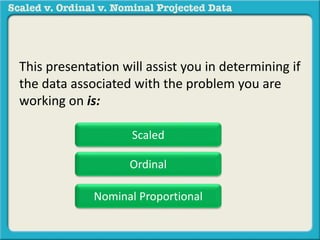
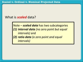
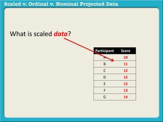
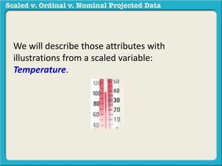
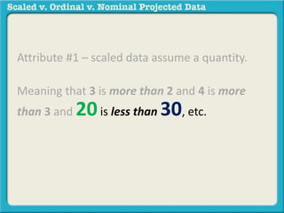
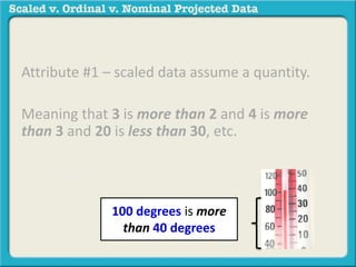
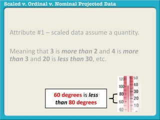
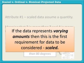
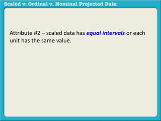
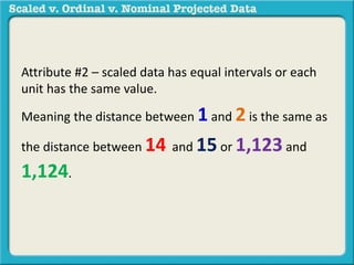
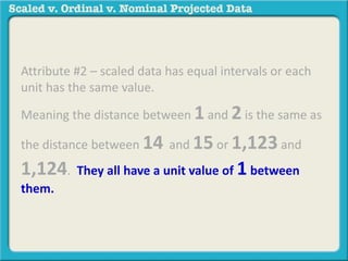
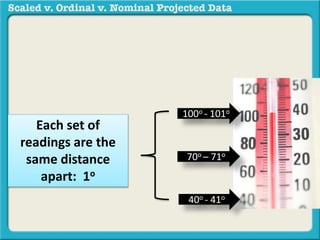
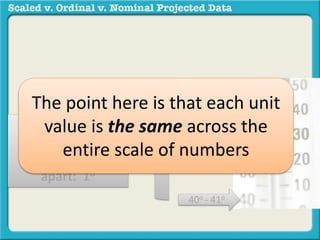
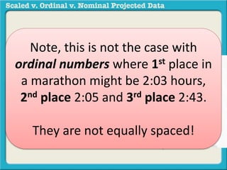
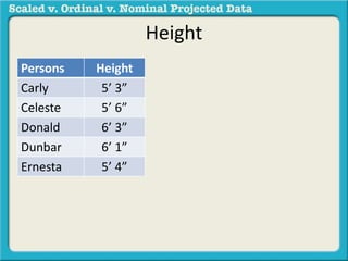
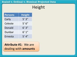
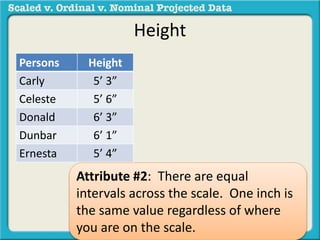
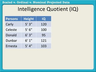
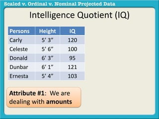
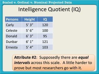
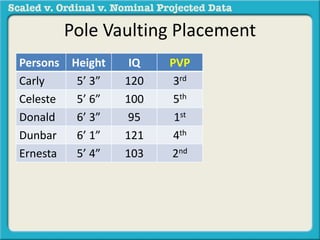
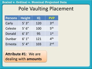
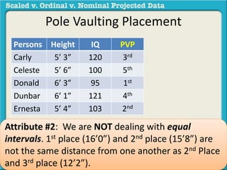
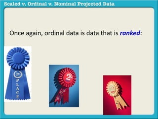
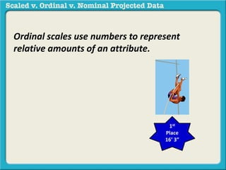
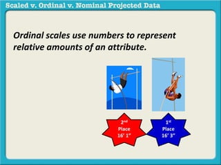
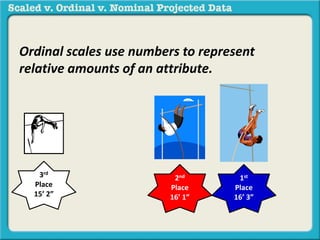
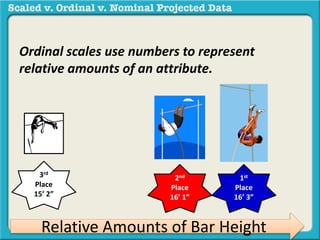
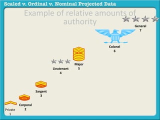
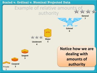
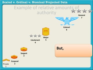
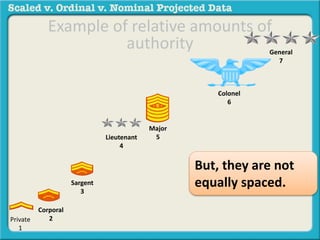
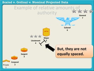
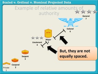
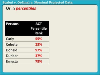
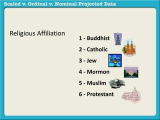
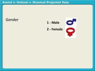
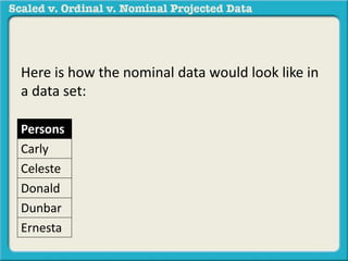
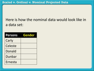
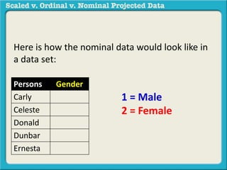
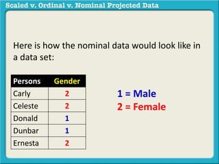
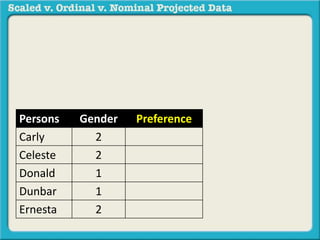
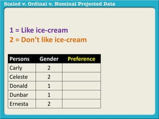
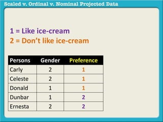
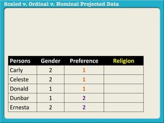
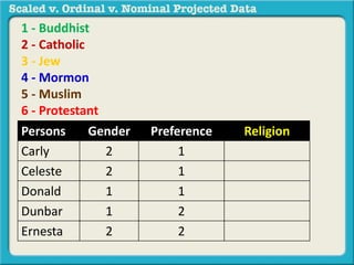
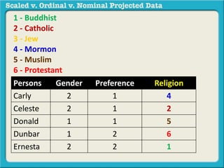
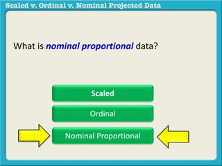
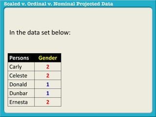
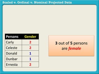
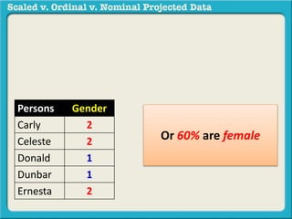
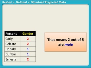
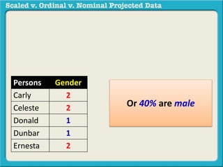
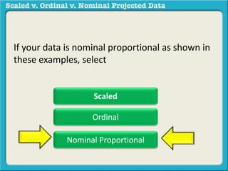
The document discusses different types of data used in statistical analysis: scaled, ordinal, and nominal data. Scaled data represents quantities where the intervals between values are equal, such as temperature or test scores. Ordinal data uses numbers to represent relative rankings, like placing in an event, but the intervals are not equal. The document uses examples to illustrate the properties of scaled and ordinal data and explains how to determine if a given data set is scaled or ordinal.

1. This presentation will assist you in determining if
the data associated with the problem you are
working on

2. This presentation will assist you in determining if
the data associated with the problem you are
working on
Participant Score
A 10
B 11
C 12
D 12
E 12
F 13
G 14

3. This presentation will assist you in determining if
the data associated with the problem you are
working on
Participant Score
A 10
B 11
C 12
D 12
E 12
F 13
G 14

4. This presentation will assist you in determining if
the data associated with the problem you are
working on is:

5. This presentation will assist you in determining if
the data associated with the problem you are
working on is:
Scaled

6. This presentation will assist you in determining if
the data associated with the problem you are
working on is:
Scaled
Ordinal

7. This presentation will assist you in determining if
the data associated with the problem you are
working on is:
Scaled
Ordinal
Nominal Proportional

8. First, a little background

9. With inferential statistics you will use either
parametric or nonparametric methods.

10. What is a parametric method?

11. Parametric methods use story telling tools like
center (what is the average height?), spread
(how big is the difference between the shortest
and tallest person?), or association (what is the
relationship between height and weight?) in a
sample to generalize to a population.

12. Parametric methods use story telling tools like
center (what is the relationship between height
and weight?) in a sample to generalize to a
population.

13. Parametric methods use story telling tools like
center (e.g., what is the average height?),
spread (how big is the difference between the
shortest and tallest person?), or association
(what is the relationship between height and
weight?) in a sample to generalize to a
population.

14. Parametric methods use story telling tools like
center (what is the average height?), spread
(how big is the difference between the shortest
and tallest person?), or association (what is the
relationship between height and weight?) in a
sample to generalize to a population.

15. Parametric methods use story telling tools like
center (what is the average height?), spread
(e.g., how big is the difference between the
shortest and tallest person?), or association
(what is the relationship between height and
weight?) in a sample to generalize to a
population.

16. Parametric methods use story telling tools like
center (what is the average height?), spread
(how big is the difference between the shortest
and tallest person?), or association (what is the
relationship between height and weight?) in a
sample to generalize to a population.

17. Parametric methods use story telling tools like
center (what is the average height?), spread
(how big is the difference between the shortest
and tallest person?), or association (e.g., what
is the relationship between height and
weight?). in a sample to generalize to a
population.

18. Parametric methods use story telling tools like
center (what is the average height?), spread
(how big is the difference between the shortest
and tallest person?), or association (e.g., what is
the relationship between height and weight?) in
a sample to generalize to a population.

19. Parametric methods use these story telling tools
(center, spread, association) in a sample

20. Parametric methods use these story telling tools
(center, spread, association) in a sample
SAMPLE

21. Parametric methods use these story telling tools
(center, spread, association) in a sample
to generalize to
SAMPLE

22. Parametric methods use these story telling tools
(center, spread, association) in a sample to
generalize to
SAMPLE

23. Parametric methods use these story telling tools
(center, spread, association) in a sample to
generalize to a population.
SAMPLE

24. Parametric methods use these story telling tools
(center, spread, association) in a sample to
generalize to a population.
SAMPLE
POPULATION

25. We ask . . .

26. We ask . . .
what is the probability that what's happening in
a sample,

27. We ask . . .
what is the probability that what's happening in
a sample,
SAMPLE:
center, spread,
association

28. We ask . . .
what is the probability that what's happening in
a sample, is happening in
SAMPLE:
center, spread,
association

29. We ask . . .
what is the probability that what's happening in
a sample, is happening in
SAMPLE:
center, spread,
association

30. We ask . . .
what is the probability that what's happening in
a sample, is happening in a population.
SAMPLE:
center, spread,
association

31. We ask . . .
what is the probability that what's happening in
a sample, is happening in a population.
SAMPLE:
center, spread,
association
POPULATION:
center, spread, association

32. To make that kind of leap (from sample to
population) requires that certain conditions are
met.

33. To make that kind of leap (from sample to
population) requires that certain conditions are
met.
Conditions or assumptions
that must be met

34. These are called parametric CONDITIONS or
ASSUMPTIONS

35. The first condition is that the data be scaled

36. What is scaled data?

37. What is scaled data?
Note – scaled data has two subcategories
(1) interval data (no zero point but equal
intervals) and
(2) ratio data (a zero point and equal
intervals)

38. What is scaled data?
For the purposes of this presentation we will
not discuss these further but just focus on
both as scaled data.

39. What is scaled data?
Participant Score
A 10
B 11
C 12
D 12
E 12
F 13
G 14

40. Scaled data is data that has a couple of
attributes.

41. We will describe those attributes with
illustrations from a scaled variable:

42. We will describe those attributes with
illustrations from a scaled variable:
Temperature.

43. Attribute #1 – scaled data assume a quantity.
Meaning that 2 is more than 3 and 4 is more
than 3 and 20 is less than 30, etc.
For example: 40 degrees is more
than 30 degrees. 110 degrees is
less than 120 degrees.

44. Attribute #1 – scaled data assume a quantity.
Meaning that 2 is more than 3 and 4 is more
than 3 and 20 is less than 30, etc.
For example: 40 degrees is more
than 30 degrees. 110 degrees is
less than 120 degrees.

45. Attribute #1 – scaled data assume a quantity.
Meaning that 3is more than 2and 4 is more than
3 and 20 is less than 30, etc.
For example: 40 degrees is more
than 30 degrees. 110 degrees is
less than 120 degrees.

46. Attribute #1 – scaled data assume a quantity.
Meaning that 3 is more than 2 and 4 is more than
3and 20 is less than 30, etc.
For example: 40 degrees is more
than 30 degrees. 110 degrees is
less than 120 degrees.

47. Attribute #1 – scaled data assume a quantity.
Meaning that 3 is more than 2 and 4 is more
than 3 and 20 is less than 30, etc.
For example: 40 degrees is more
than 30 degrees. 110 degrees is
less than 120 degrees.

48. Attribute #1 – scaled data assume a quantity.
Meaning that 3 is more than 2 and 4 is more
than 3 and 20 is less than 30, etc.
For example: 40 degrees is more
than 30 degrees. 110 degrees is
less than 120 d1e0g0 rdeeegsr.ees is more
than 40 degrees

49. Attribute #1 – scaled data assume a quantity.
Meaning that 3 is more than 2 and 4 is more
than 3 and 20 is less than 30, etc.
For example: 40 degrees is more
than 30 degrees. 110 degrees is
less than 120 de6g0r deeegsr.ees is less
than 80 degrees

50. Attribute #1 – scaled data assume a quantity.
Meaning that 3 is more than 2 and 4 is more
than 3 and 20 is less than 30, etc.
If the data represents varying
amounts then this is the first
requirement for data to be
For example: 40 degrees is more
than 30 degrees. 110 degrees is
less than 120 de6g0r deeegsr.ees is less
considered - scaled.
than 80 degrees

51. Attribute #2

52. Attribute #2 – scaled data has equal intervals or each
unit has the same value.

53. Attribute #2 – scaled data has equal intervals or each
unit has the same value.
Meaning the distance between 1 and 2 is the same as
the distance between 14 and 15 or 1,123 and
1,124.

54. Attribute #2 – scaled data has equal intervals or each
unit has the same value.
Meaning the distance between 1 and 2 is the same as
the distance between 14 and 15 or 1,123 and
1,124. They all have a unit value of 1 between
them.

55. In our temperature example:

56. 100o - 101o
70o – 71o
40o - 41o
Each set of
readings are the
same distance
apart: 1o

57. The point here is that each unit
100o - 101o
value is the same across the
entire scale of numbers
70o – 71o
40o - 41o
Each set of
readings are the
same distance
apart: 1o

58. Note, this is not the case with
ordinal numbers where 1st place in
a marathon might be 100o 2:- 101o
03 hours,
2nd place 2:05 and 3rd place 2:43.
70o – 71o
40o - 41o
Each set of
readings are the
same distance
apart: 1o
They are not equally spaced!

59. What does a scaled data set look like?

60. Here are some examples:

61. Height

62. Height
Persons Height
Carly 5’ 3”
Celeste 5’ 6”
Donald 6’ 3”
Dunbar 6’ 1”
Ernesta 5’ 4”

63. Height
Persons Height
Carly 5’ 3”
Celeste 5’ 6”
Donald 6’ 3”
Dunbar 6’ 1”
Ernesta 5’ 4”
Attribute #1: We are
dealing with amounts

64. Height
Persons Height
Carly 5’ 3”
Celeste 5’ 6”
Donald 6’ 3”
Dunbar 6’ 1”
Ernesta 5’ 4”
Attribute #2: There are equal
intervals across the scale. One inch is
the same value regardless of where
you are on the scale.

65. Intelligence Quotient (IQ)

66. Intelligence Quotient (IQ)
Persons Height IQ
Carly 5’ 3” 120
Celeste 5’ 6” 100
Donald 6’ 3” 95
Dunbar 6’ 1” 121
Ernesta 5’ 4” 103

67. Intelligence Quotient (IQ)
Persons Height IQ
Carly 5’ 3” 120
Celeste 5’ 6” 100
Donald 6’ 3” 95
Dunbar 6’ 1” 121
Ernesta 5’ 4” 103
Attribute #1: We are
dealing with amounts

68. Intelligence Quotient (IQ)
Persons Height IQ
Carly 5’ 3” 120
Celeste 5’ 6” 100
Donald 6’ 3” 95
Dunbar 6’ 1” 121
Ernesta 5’ 4” 103
Attribute #2: Supposedly there are equal
intervals across this scale. A little harder to
prove but most researchers go with it.

69. Pole Vaulting Placement

70. Pole Vaulting Placement
Persons Height IQ PVP
Carly 5’ 3” 120 3rd
Celeste 5’ 6” 100 5th
Donald 6’ 3” 95 1st
Dunbar 6’ 1” 121 4th
Ernesta 5’ 4” 103 2nd

71. Pole Vaulting Placement
Persons Height IQ PVP
Carly 5’ 3” 120 3rd
Celeste 5’ 6” 100 5th
Donald 6’ 3” 95 1st
Dunbar 6’ 1” 121 4th
Ernesta 5’ 4” 103 2nd
Attribute #1: We are
dealing with amounts

72. Pole Vaulting Placement
Persons Height IQ PVP
Carly 5’ 3” 120 3rd
Celeste 5’ 6” 100 5th
Donald 6’ 3” 95 1st
Dunbar 6’ 1” 121 4th
Ernesta 5’ 4” 103 2nd
Attribute #2: We are NOT dealing with equal
intervals. 1st place (16’0”) and 2nd place (15’8”) are
not the same distance from one another as 2nd Place
and 3rd place (12’2”).

73. Based on this explanation is your data scaled?

74. If your data is scaled as shown in these
examples, select

75. If your data is scaled as shown in these
examples, select
Scaled
Ordinal
Nominal Proportional

76. We have now demonstrated scaled data and
given you a brief introduction to ordinal data.

77. Once again, ordinal data is data that is ranked:

78. Once again, ordinal data is data that is ranked:

79. In other words,

80. Ordinal scales use numbers to represent
relative amounts of an attribute.

81. Ordinal scales use numbers to represent
relative amounts of an attribute.
1st
Place
16’ 3”

82. Ordinal scales use numbers to represent
relative amounts of an attribute.
1st
Place
16’ 3”
2nd
Place
16’ 1”

83. Ordinal scales use numbers to represent
relative amounts of an attribute.
1st
Place
16’ 3”
2nd
Place
16’ 1”
3rd
Place
15’ 2”

84. Ordinal scales use numbers to represent
relative amounts of an attribute.
3rd
Place
15’ 2”
2nd
Place
16’ 1”
1st
Place
16’ 3”
Relative Amounts of Bar Height

85. Example of relative amounts of
authority

86. Corporal
2
Sargent
3
Lieutenant
4
Major
5
Colonel
6
General
7
Private
1
Example of relative amounts of
authority

87. Example of relative amounts of
Corporal
2
Sargent
3
Lieutenant
4
Major
5
Colonel
6
General
7
Private
1
Notice how we are
dealing with
amounts of
authority
authority

88. Example of relative amounts of
Corporal
2
Sargent
3
Lieutenant
4
Major
5
Colonel
6
General
7
Private
1
But,
authority

89. Example of relative amounts of
Corporal
2
Sargent
3
Lieutenant
4
Major
5
Colonel
6
General
7
Private
1
But, they are not
equally spaced.
authority

90. Example of relative amounts of
Corporal
2
Sargent
3
Lieutenant
4
Major
5
Colonel
6
General
7
Private
1
But, they are not
equally spaced.
authority

91. Example of relative amounts of
Corporal
2
Sargent
3
Lieutenant
4
Major
5
Colonel
6
General
7
Private
1
But, they are not
equally spaced.
authority

92. You can tell if you have an ordinal data set when
the data is described as ranks.

93. You can tell if you have an ordinal data set when
the data is described as ranks.
Persons Pole Vault
Placement
Carly 3rd
Celeste 5th
Donald 1st
Dunbar 4th
Ernesta 2nd

94. Or in percentiles

95. Or in percentiles
Persons ACT
Percentile
Rank
Carly 55%
Celeste 23%
Donald 97%
Dunbar 37%
Ernesta 78%

96. If your data is ranked as shown in these
examples, select

97. If your data is ranked as shown in these
examples, select
Scaled
Ordinal
Nominal Proportional

98. Finally, let’s see what data looks like when it is
nominal proportional:

99. Nominal data is different from scaled or ordinal,

100. Nominal data is different from scaled or ordinal,
because they do not deal with amounts

101. Nominal data is different from scaled or ordinal,
because they do not deal with amounts nor
equal intervals.

102. For example,

103. Nationality is a variable that does not have
amounts nor equal intervals.

104. 1 = Canadian
2 = American

105. Being Canadian is not numerically or
quantitatively more than being
1 = Canadian
2 = American
American

106. The numbers 1 and 2 do not represent
amounts. They are just a way to
distinguish the two groups numerically.
1 = Canadian
2 = American

107. We could have just as easily used 1s for
Americans and 2s for Canadians

108. We could have just as easily used 1s for
Americans and 2s for Canadians
1 = Canadian
2 = American

109. We could have just as easily used 1s for
Americans and 2s for Canadians
1 = American
2 = Canadian

110. Other examples:

111. Religious Affiliation

112. Religious Affiliation
1 - Buddhist
2 - Catholic
3 - Jew
4 - Mormon
5 - Muslim
6 - Protestant

113. Gender

114. Gender
1 - Male
2 - Female

115. Preference

116. Preference:
1. People who prefer chocolate ice-cream

117. Preference:
1. People who prefer chocolate ice-cream
2. People who dislike chocolate ice-cream

118. Pass/Fail

119. Pass/Fail
1. Those who passed the test

120. Pass/Fail
1. Those who passed the test
2. Those who failed the test

121. The word “Nom” in “nominal” means “name”.

122. The word “Nom” in nominal means “name”.
Essentially we are using data to name, identify,
distinguish, classify or categorize.

123. Other names for nominal data are categorical or
frequency data.

124. Here is how the nominal data would look like in
a data set:

125. Here is how the nominal data would look like in
a data set:
Persons
Carly
Celeste
Donald
Dunbar
Ernesta

126. Here is how the nominal data would look like in
a data set:
Persons Gender
Carly
Celeste
Donald
Dunbar
Ernesta

127. Here is how the nominal data would look like in
a data set:
Persons Gender
Carly
Celeste
Donald
Dunbar
Ernesta
1 = Male
2 = Female

128. Here is how the nominal data would look like in
a data set:
Persons Gender
Carly 2
Celeste 2
Donald 1
Dunbar 1
Ernesta 2
1 = Male
2 = Female

129. Persons Gender Preference
Carly 2
Celeste 2
Donald 1
Dunbar 1
Ernesta 2

130. 1 = Like ice-cream
2 = Don’t like ice-cream
Persons Gender Preference
Carly 2
Celeste 2
Donald 1
Dunbar 1
Ernesta 2

131. 1 = Like ice-cream
2 = Don’t like ice-cream
Persons Gender Preference
Carly 2 1
Celeste 2 1
Donald 1 1
Dunbar 1 2
Ernesta 2 2

132. Persons Gender Preference
Carly 2 1
Celeste 2 1
Donald 1 1
Dunbar 1 2
Ernesta 2 2
Religion

133. Persons Gender Preference
Carly 2 1
Celeste 2 1
Donald 1 1
Dunbar 1 2
Ernesta 2 2
Religion
1 - Buddhist
2 - Catholic
3 - Jew
4 - Mormon
5 - Muslim
6 - Protestant

134. Persons Gender Preference
Carly 2 1
Celeste 2 1
Donald 1 1
Dunbar 1 2
Ernesta 2 2
Religion
4
2
5
6
1
1 - Buddhist
2 - Catholic
3 - Jew
4 - Mormon
5 - Muslim
6 - Protestant

135. Now that we know what nominal data is,

136. What is nominal proportional data?

137. What is nominal proportional data?
Scaled
Ordinal
Nominal Proportional

138. Nominal proportional data is simply the
proportion of individuals who are in one
category as opposed to another.

139. For example,

140. In the data set below:

141. In the data set below:
Persons Gender
Carly 2
Celeste 2
Donald 1
Dunbar 1
Ernesta 2

142. Persons Gender
Carly 2
Celeste 2
Donald 1
Dunbar 1
Ernesta 2
3 out of 5 persons
are female

143. Persons Gender
Carly 2
Celeste 2
Donald 1
Dunbar 1
Ernesta 2
Or 60% are female

144. Persons Gender
Carly 2
Celeste 2
Donald 1
Dunbar 1
Ernesta 2
That means 2 out of 5
are male

145. Persons Gender
Carly 2
Celeste 2
Donald 1
Dunbar 1
Ernesta 2
Or 40% are male

146. In such cases you may not see a data set,

147. you may just see a question like this:

148. A claim is made that four out of five veterans (or
80%) are supportive of the current conflict.
After you sample five veterans you find that
three out of five (or 60%) are supportive. In
terms of statistical significance does this result
support or invalidate this claim?

149. If you were to put these results in a data set it
would look like this:

150. Veterans
A
B
C
D
E

151. Veterans Supportive
A
B
C
D
E

152. Veterans Supportive
A
B
C
D
E
1 = supportive
2 = not supportive

153. Veterans Supportive
A 2
B 2
C 1
D 1
E 1
1 = supportive
2 = not supportive

154. If the question is stated in terms of percentages
(e.g., 60% of veterans were supportive), then
that percentage is nominal proportional data
Veterans Supportive
A 2
B 2
C 1
D 1
E 1
1 = supportive
2 = not supportive

155. If your data is nominal proportional as shown in
these examples, select

156. If your data is nominal proportional as shown in
these examples, select
Scaled
Ordinal
Nominal Proportional

157. That concludes this explanation of scaled,
ordinal and nominal proportional data.