Download as PDF, PPTX

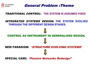
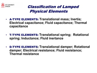
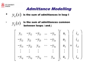
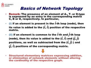
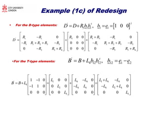
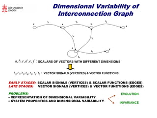
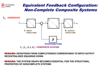
![The RC, RL Matrix PencilThe RC, RL Matrix Pencil
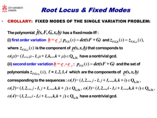
•• PROPERTIES OF THE RC, OR RL NETWORK OPERATORPROPERTIES OF THE RC, OR RL NETWORK OPERATOR
[ ]s
kxk
t t
sF + G
(sF + G) (sF + G) 0 F G 0
F = F 0, G = G 0
Given the network pencil we have the following properties :
(i) is regular, ie det and ker{ } ker{ } = { }
(ii) and all eigenvalues are real and non - posi
1 1fk
}
}
:kxk
1
1,
sF + G
sF + G (sF + G) F
F G 0 T 0
tive
(iii) All finite eigenvalues are real and index{
(iv) If index{ then deg{det } = rank{ }
(v) If ker{ } ker{ } = { }, and diag{ },,...,
0
{ } fk k k
t
T sF + G T = sI + sI sIblock - diag{ } ](https://image.slidesharecdn.com/passive-network-redesign-ntua-jan-13-13-01-131-140417085604-phpapp01/85/Passive-network-redesign-ntua-19-320.jpg)
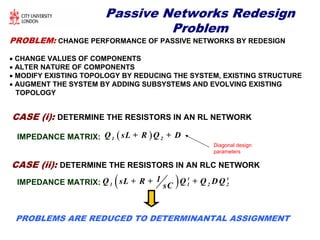
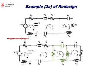
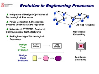
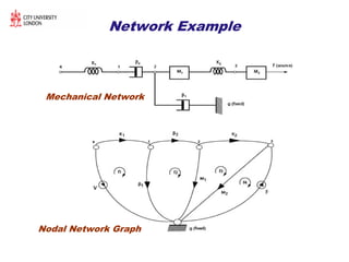
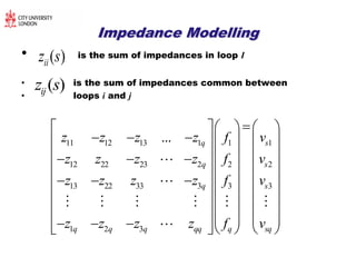
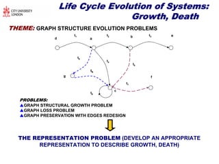
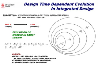
![AA--D & TD & T--D Networks: singleD Networks: single
Parameter PerturbationsParameter Perturbations
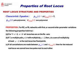
• PROBLEM: [ ]s
kxk
'
sF + G
F F + F(x,b), G = G + G(x,b),
F(x,b),G(x,b) = xbb
Given investigate the effect
of perturbations on the pencil of the type :
where
, ,
t
i i jb = e b = e e
f(s,F,G, x,b)= det(s(F + F(x,b))+ G)
f(s,F
or
Study the determinantal assignment problems
,G, x,b)= det(sF + G + (G(x,b))](https://image.slidesharecdn.com/passive-network-redesign-ntua-jan-13-13-01-131-140417085604-phpapp01/85/Passive-network-redesign-ntua-26-320.jpg)
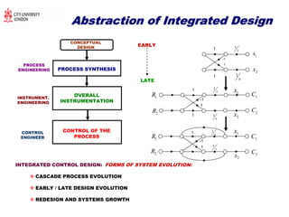
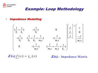
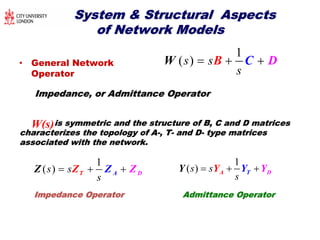
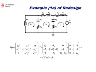
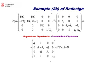
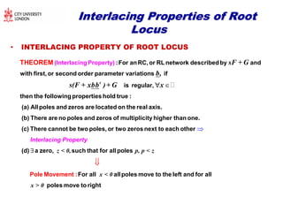
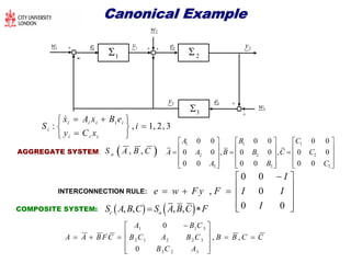
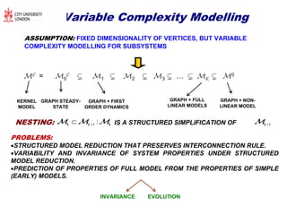
![The Network CharacteristicThe Network Characteristic
PolynomialPolynomial (a)(a)
• Problem Formulation: Binet-Cauchy Theorem
( )
[ ]
i
i j
k
k
-k b = e
b = e e
f(s,F,G, x,b)= det s(F + F(x,b))+ G =
I
= det sF + G, I
sF(x,b)
(second order
(firs
variatio
node or loop graph a t order variation)nd or
n)
Assume :
2k
k
2k1
k
x
[ ]
t
kt
k k k
g(s,F,G) p(s, x,b)
I
g(s,F,G) = C sF + G, I , p(s, x,b) = C
sF(x,b)
g(s,F,G) :
p(s, x,b) : Grass
Grassmann vector of
mann vector of the
the netw
structu
ork
ralperturbation](https://image.slidesharecdn.com/passive-network-redesign-ntua-jan-13-13-01-131-140417085604-phpapp01/85/Passive-network-redesign-ntua-27-320.jpg)
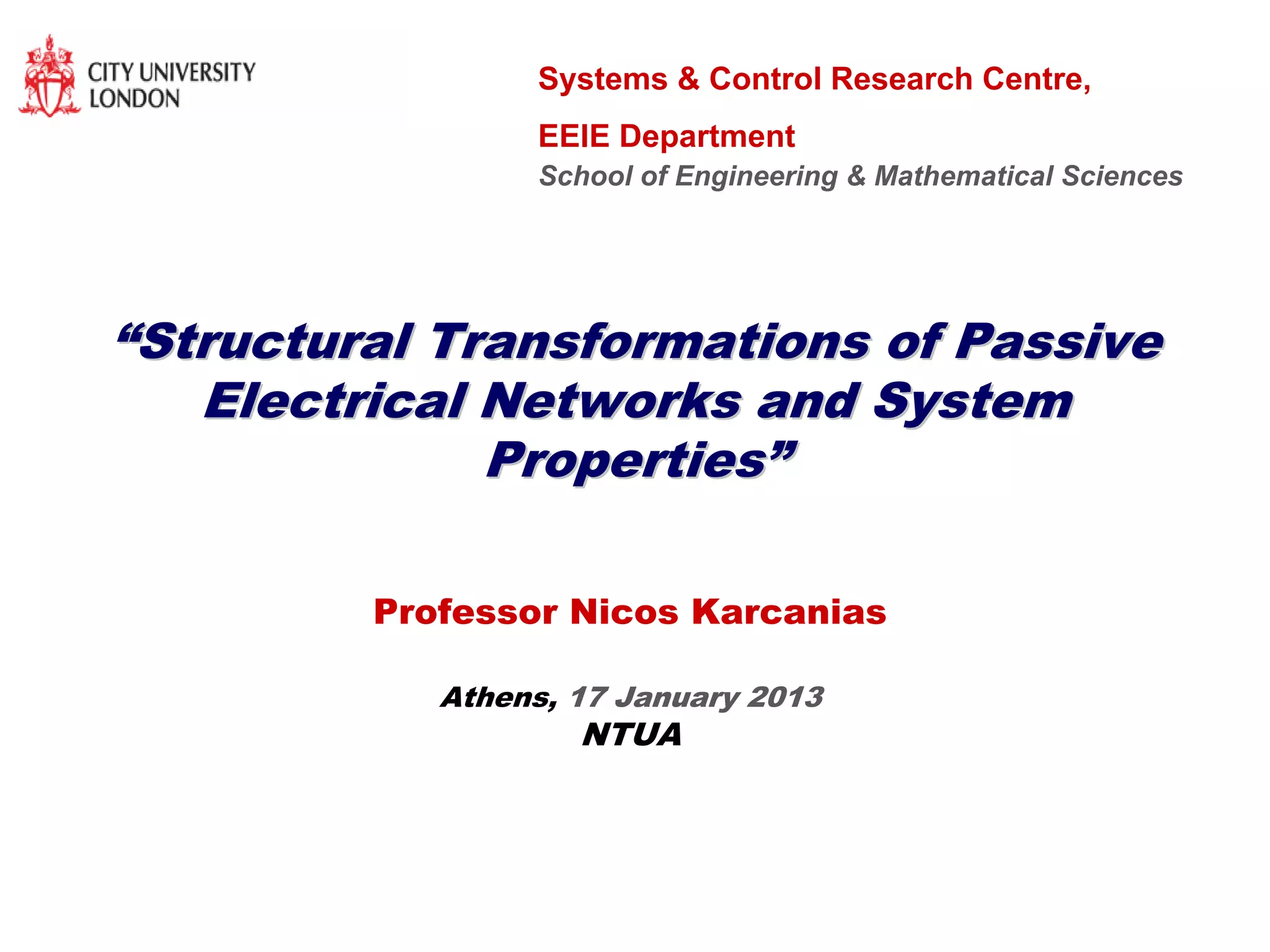
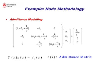
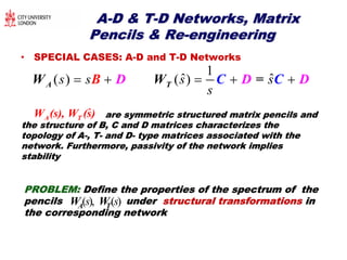
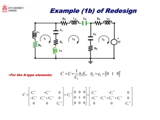
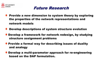
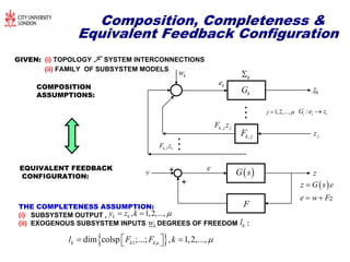
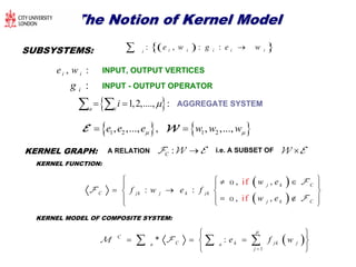
![The Network CharacteristicThe Network Characteristic
PolynomialPolynomial (b)(b)
• Lemma: Grassmann vector of Structural Perturbation
, ,
( )=( , ( )
i
sx
sign
k,2k
[ ],
) Q
( ) ( ) ( )
j
1,0,..,a 0,...,0 a
1,.., -1, +1,k,...k+
b= e
b=
p(s,x,b),
p s,x,e =
p(s,x,b)e e
firstorder variation
secondorder varia
hasthestructure:
tion : ha-
:
1 2 3 4,
( ) , r= ( )
( )=( , ( )=(
i
r
j j i j j j
r sx r
k,2k
[ ]
) Q
( ) , , ,j ( ) ( ) ( ) ( )
( )
1,0,..,a 0,...,0,a 0,...,0,a 0,...,0,a 0,...,0
a 1,2,3,4 1
1 1,2,.., -1, +1,...,k,k+ 2 1,2,.., -1, +1,...,k,k+
p s,x,e e =
sthestructure:
-
,
( )=( , ( )=(i i i i j
k,2k
k,2k k,2k
) Q
) Q ) Q3 1,2,..,i -1, +1,...,k,k+ 4 1,2,.., -1, +1,...,k,k+](https://image.slidesharecdn.com/passive-network-redesign-ntua-jan-13-13-01-131-140417085604-phpapp01/85/Passive-network-redesign-ntua-28-320.jpg)
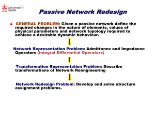
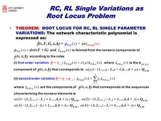
![The Network CharacteristicThe Network Characteristic
PolynomialPolynomial (c)(c)
• LEMMA: GRASSMANN VECTORS OF STRUCTURAL
PERTURBATIONS
, ,
( )=( , ( )
i
sx
sign
k,2k
[ ],
) Q
( )
firstorder variation
secondorder
hasthestructure:
variation ha:-
:
( ) ( )
j
1,0,..,a 0,...,0 a
1,.., -1, +1,k,...k+
p(s,x,b),
p s,x,e =
p(s,
b= e
b= e e x,b)
1 2 3 4,
( ) , r= ( )
( )=( , ( )=(
i
r
j j i j j j
r sx r
k,2k
[ ]
) Q
( ) , , ,
sthestructure:
- j ( ) ( ) ( ) ( )
( )
1,0,..,a 0,...,0,a 0,...,0,a 0,...,0,a 0,...,0
a 1,2,3,4 1
1 1,2,.., -1, +1,...,k,k+ 2 1,2,.., -1, +1,...,k,k+
p s,x,e e =
,
( )=( , ( )=(i i i i j
k,2k
k,2k k,2k
) Q
) Q ) Q3 1,2,..,i -1, +1,...,k,k+ 4 1,2,.., -1, +1,...,k,k+](https://image.slidesharecdn.com/passive-network-redesign-ntua-jan-13-13-01-131-140417085604-phpapp01/85/Passive-network-redesign-ntua-29-320.jpg)


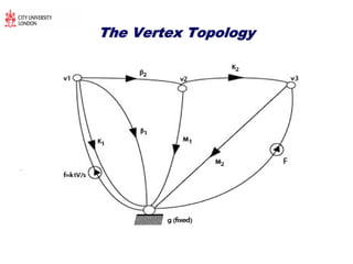
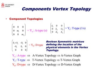
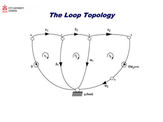
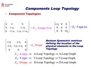
The document discusses structural transformations in passive electrical networks, focusing on redesigning components and their topologies to enhance dynamic behavior. It outlines various types of elements, the modeling of networks, and specifies challenges in network representation and transformation. The content emphasizes the importance of integrated design and control in evolving engineering processes related to energy systems and technology networks.


![Deformable DETR Review [CDM]](https://cdn.slidesharecdn.com/ss_thumbnails/deformabledetrreviewcdm-201113070345-thumbnail.jpg?width=640&height=640&fit=bounds)