Downloaded 327 times


![, = [ − − − − ]
[
,
,
,
, ]
Application of Bilinear Surfaces
Bilinear patches are extensively used in 2-D finite element analysis (FEA). In FEA, an engineering structure is
defined by several bilinear surfaces elements , which are created by joining points on the structure’s geometry,
called nodes. The nodes are connected to other nodes to create quadrilateral surfaces. Points not lying on the
nodes are calculated by interpolation. Thus, the entire structure is completely defined by the nodes and the
bilinear surfaces.
Drawbacks of Bilinear Surfaces
Bilinear surfaces have a very limited use, mainly, for FEA. Since only 4 points can be used in the interpolation, the
smoothness of the generated surface is limited. Additionally, there is no flexibility to control shapes of the
surface, unlike the sweeped surfaces.
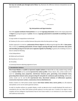
4. Interpolated Surfaces – Coons Patch
A linear interpolation between four bounded curves is used to generate a Coons surface, also called as Coons patch.
The method is credited to S. Coons who developed this concept for generating a surface.
Linear interpolation between the boundary curves P(0,v), P(u,0), P(1,v) , and P(u,1) gives the equation
, = − , + , + , + − ,
The above equation gives wrong values at the corners (u,v = 0 and 1). For example, substituting the values of u
and v we get,
, = , + , = ,
, = ,
Which are obviously wrong values, therefore, the coons patch is created by modification of the interpolation
equation, where the corners are subtracted. The modified interpolation equation is given as,
, = − , + , − , + − , − − − , − − ,
− − , − ,
For computational purposes, it is more convenient to write this equation as,](https://image.slidesharecdn.com/cadunit-42016-161018092044/85/Surfaces-6-320.jpg)
![, = [ − − ]
[
,
,
,
, ]
− � .
−[ − − − − ]
[
,
,
,
, ]
− � � �
Which gives,
, = [ − ] [
− , − , ,
− , − , ,
, ,
] [
−
]
Other interpolated surfaces include the Parametric Cubic patches.
Applications
Coon’s Surface is easy to create, and therefore, many 2-D CAD packages utilize it for generating models. However,
it has only a limited application since the surface is inflexible and cannot create very smooth surfaces. It would be
very difficult to produce a smooth automobile fender using the Coons surface. Several CAD software, including,
AutoCAD uses this surface for generating surfaces between 4-bounded edges.
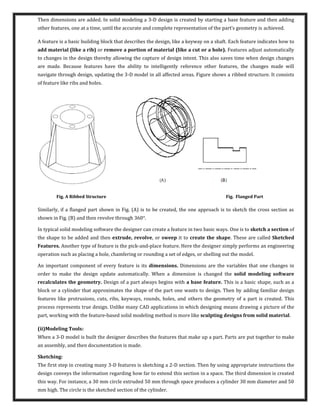
5. Linearly Sweeped Surfaces
A Sweeped Surface is generated when a curve is parametrically translated or rotated. In CAD, a surface is
represented by a series of curves, which are parametrically generated at various instances. For example, a
cylindrical surface is generated when a circular arc is translated up to the given dimension using a parameter t,
where t varies as, ≤ t ≤ .
In the figure shown, the cylindrical surface is generated when a circular arc is translated a distance L, with the
interim instances at t = 0.1, 0.2, 0.3, 1. Here, the parameter t is given 10 values, and therefore, the surface of the
cylinder is represented by 10 circular curves. The appearance of the surface improves as the parameter t varies at
smaller intervals. Thus, if t is varied with Δt = . , there will be 100 circular curves representing the surface.
A surface is an extension of a curve. The parametric representation of a curve is given by a single-vector equation
of the form:
= [ ]
Here, only one parametric variable or one degree of freedom is needed. Whereas, a surface representation requires
two parametric variables, and the equation is given as:
, = [ , , , ]
Tracing a point in the s and t directions, as shown in the figure on the next page, generates a surface. One
parameter variable is kept constant while varying the other one. A series of curves is created along the s and t](https://image.slidesharecdn.com/cadunit-42016-161018092044/85/Surfaces-7-320.jpg)
![directions. For example, constraining the parameters s and t between zero and 1, the set of curves generated along
the s direction is,
, , . , , . , … … … . ,
and the other set of curves along the t direction is,
, , , . , , . … … … . ,
Thus, creation of a surface requires creation of the multiple curves that constitute it. This concept can be applied to
both, the surface that has an analytical formulation (conic sections) and to a free-form surface (Bezier, B-spline).
6. Revolved Surfaces (Circular Sweep)
Surface of revolution is obtained by rotating a plane-curve around an axis. In the figure shown, line AB is rotated
about the z-axis through an angle of 2π radians, generating a cylinder. A line or curve when revolved can generate
all kinds of surfaces, based on the condition of rotation. Any point on the surface is a function of two parameters t
and θ. Here, t describes the entity to be rotated and θ represents the angle of rotation. In general, a point on line
AB (lying in the xz-plane) is represented by [x(t), 0, z(t)] and, when rotated by θ radians, it becomes [x t cosθ,
x t sinθ, z t ].
In general, the point matrix gives a point on the surface of revolution obtained by rotation around the z-axis,
, � = [ � � � ]
In matrix form the equation can be written as,
, � = [ ]
[
� � �
]](https://image.slidesharecdn.com/cadunit-42016-161018092044/85/Surfaces-8-320.jpg)
![Note: The above rotation matrix is equivalent to the rotational transformation matrix studied earlier, which is,
[
� � �
]
= −
[
� � �
− � � �
]
Thus, the generated surface is a rotational transformation of a line (or curve), except θ is not constant, but has
values, ≤ θ ≤ π.
Example: Generate the conical surface obtained by rotation of the line segment AB around the z-axis with, A = (1,
0, 1) and B = (7, 0, 7).
Solution: Line AB can be represented in parametric form as:
= [ ]
and the parametric equation of a line is,
= + −
based on this equation, the coordinates of a of point on the line are given as,
= + − = + ; = ; = + − = +
The equation of the surface as given above is,
, � = [ � � � ] = [ + � + � � + ]
Any point on the surface can be located by substituting t and θ values in the above equation, e.g.: at t = .4 and θ =
π/2 radians
. , �/ = [ + . �/ + . � �/ + . ] = [ . . ]
which is the point on the surface at (0.4, π/2)
Example: Generate a Torus by rotating a circle of radius r and the center at (a,0,0) about the z-axis.
Solution: Rotating a circle contained in the x z plane around the z-axis can generate a torus. The center of the
circle has coordinates (a, 0, 0) and equation of the circle in parametric form is given as;
� = [ + � , , � � ]
The torus is represented by,
�, � = {[ + � �], [ + � � �], � �}](https://image.slidesharecdn.com/cadunit-42016-161018092044/85/Surfaces-9-320.jpg)
![In this case, the parameters are φ and θ.
7. Circular Sweep of a Synthetic Curve
Equation of a synthetic curve (free-form curve), is given as,
= [ ][�][�]
The surface of revolution is then given by,
, � = [ ][�][�][ ]�
= [ ][ ]�
Where, Q (t, θ is the equation of the curve, and [Tr]θ is the rotation matrix about the z-axis.
Note: To rotate the curve about the axis, we will have to use the translation and rotation matrices.
Example: A cubic Bezier curve is defined by the control points: P1 (1,0,2), P2 (3,0,4), P3 (2,0,6), P4 (5,0,7). Find the
surface of revolution obtained by revolving the curve about the z-axis and calculate the point on the surface at t =
0.5, θ = π/4 rad.
Solution: The cubic Bezier curve is given by the equation,
= [ ][�][�] = [ ]
[
− −
−
−
] [ ]
Substituting the coordinates of the points, we get
= [ ]
[
− −
−
−
] [ ]
The surface of revolution is:
, � = [ ]
[
− −
−
−
] [ ] [
� � �
]
≤ � ≤ � ; ≤ ≤
For t = 0.5 and θ = π/4, the surface equation is,
, � = [ . . . ]
[
− −
−
−
] [ ] [
�/ � �/
]
= [ . . . ]
8. Creating a Surface by Parametric Sweeping
In the examples given above, sweeping a curve parametrically generated the surfaces. In parametric sweeping
procedure, a surface is generated through the movement of a line or a curve along or around a defined path. The
curve is sweeped as the sweep parameter is varied from the values of 0 to 1, creating several instances of the curve
along the sweep path. In general, the equation of the surface can be given as,](https://image.slidesharecdn.com/cadunit-42016-161018092044/85/Surfaces-10-320.jpg)
![, =
Where, P(t) is the parametric equation of a curve and T(s) is the sweep transformation based on the shape of
the path. The sweep transformation can consist of translation, scaling, rotation or a combined transformation. If
the path is a straight line, the points along the path on the line can be represented by,
= ; = ; =
and T(s) is given as,
=
[ ]
Where, a, b, c are coordinate values, and ≤ s ≤
This is equivalent to a three-dimensional translation of a curve with several traces generated along the path,
controlled by how the parameter s is varied.
Example: Consider the Bezier curve defined by the control points P1 = (0,5,0), P2 = (3,4,0), P3 = (2,0,0), and P4 =
(5,0,0). Translate the curve five units along the z-axis to generate a swept surface.
Solution:
, = [ ][ ]
substituting the numbers, we get,
, = [ ]
[
− −
−
−
] [ ] [ ]
Substituting the value of s and solving the matrices can calculate any point on the surface.
9. Creating a Surface by Sweeping a Polygon
Any polygon can be sweeped around a given path to generate a surface. The equation of the surface is given as,
, = [ ][ ]
Where, [P] is the point matrix, and T(s) is the transformation matrix.
Example: Sweep (rotate) the triangle A (2, 2), B (5, 7), C (-2,-5) around x-axis and generate the surface
Solution:
, = [ ][ ] = [
− −
]
[
� � �
− � � �
]
Note: The value of n locates various positions on the swept surface.
10. Creating a Parametric Cubic Patch
Parametric cubic patch or surface is generated by four boundary curves; the curves are parametric cubic
polynomials. The equation of a parametric cubic curve was defined earlier as:](https://image.slidesharecdn.com/cadunit-42016-161018092044/85/Surfaces-11-320.jpg)
![= [ ]
[
−
− − −
] [
′
′
]
[
−
− − −
]
= � � = a�d
[
′
′
]
= � � �
Where P(0) = Coordinates of the first point at t = 0
P(1) = coordinates of the last point at t = 1
P’ = values of the slopes in x, y, z directions at t = 0
P’ = values of the slopes in x, y, z directions at t = 1
Analogous to a cubic curve, a parametric cubic surface can be defined by 16 points:
- 4 points for coordinates of the corner points
- 8 points for slopes in the s & t directions
- 4 points for twist vectors (second derivatives)
Using a procedure similar to the one carried out in the derivation of the cubic curve, we can derive the geometric
coefficient matrix for the surface, which is given as,
Which can be broken into 4 groups as
Twist vectors, not shown here, are the partial derivatives: dPs/dt & dPt/ds. These vectors control the internal
shape of the surface. With the geometric coefficient matrix defined, the equation of the surface can be written as,
. = [ ][�] [ ] [� ] [ ]
Where: [s] = [s3 s2 s1]
[M]H = [Constant matrix for n = 3 ]
[MH]T = Transpose of [M]H
[G]H = Geometry matrix as defined by the 16 points, and](https://image.slidesharecdn.com/cadunit-42016-161018092044/85/Surfaces-12-320.jpg)
![[ ] =
[ ]
Example: A parametric cubic surface is defined by its Cartesian components as follows:
, = [ ]
[ − ] [ ]
, = [ ]
[ ] [ ]
, = [ ]
[ ] [ ]
Obtain the normal vector at the point where s = ½, t = ½
Solution:
� , = [ ][�]�[�]�[��] [ ] = [ , , , ]
� , = [ ][�]�[ ]
����� [ ] = [�] [ ] [� ]
N���al ��ct��, =
����� =
�
; =
�
, = [ ]
[ − ] [ ]
, = [ ]
[ − ] [ ]
, = [ ]
[ − ] [ ]
at s = 0.5 & t = 0.5](https://image.slidesharecdn.com/cadunit-42016-161018092044/85/Surfaces-13-320.jpg)
![, = . ; , = .
similarly,
, = . ; , = . ; , = . ; , = .
� , = [ . . . ] ; � , = [ . . . ]
= � . , . × � . , . = [ . . .
. . .
] = − . − . + .
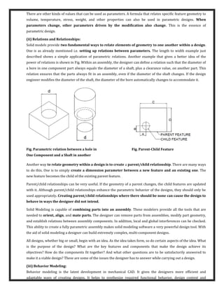
11. Bezier Surface
Just as parametric cubic curves are extended to parametric cubic patches, Bezier Curves may be extended to
Bezier Surface Patch. While the surface passes through the four corner points, the control points control all other
points on the surface. Using the placement of these points to specify edge slope is more intuitive than determining
the parametric slopes and twist vectors for the parametric cubic curve surface.
Bezier Surface, as a result, is easier to use because the control points themselves approximate the location of the
desired surface. Bezier surfaces can be generated with any order of the Bezier curve. Two surface patches can be
joined and the two surfaces do not have to be of the same order, one can be cubic and the other a quadratic.
Blending Bezier Patches with slope continuity requires that (1) control points on the common edges be shared
and (2) three control points – one on the edge and ones on the either sides of the edge – form a straight line, as
shown in the figure below.
Figure: Two blended Bezier patches. Control points P41, P42, P43 and P44 are shared by both patches. Slope
continuity between the two patches is maintained by having each group of three control points which cross the
shared edge (P31, P41, P51 etc.) lie on straight line
In Bezier Surface:
The surface takes the general shape of the control points.
The surface is contained within the convex hull of the control points.
The corner of the surface and the corner control points are coincident.
General Equation of the Bezier surface is given as,
, = � � � , , ,
≤ s, t ≤
Vi,j defines the control points
Bi,n(s) & Bj,m(t) are the Bernstein blending functions in the s and t directions.
In matrix form, the Bezier surface can be represented by,](https://image.slidesharecdn.com/cadunit-42016-161018092044/85/Surfaces-14-320.jpg)
![, = [ ][�] [�] [� ] [ ]
For a cubic surface this equation reduces to:
, = [ ]
[
− −
− −
]
[
, , , ,
, , , ,
, , , ,
, , , , ]
×
[
− −
− −
] [ ]
Note that, to represent a cubic Bezier surface, 16 control points must be specified, and several Bezier surfaces can
be combined to create a complex surface.
Geometric Modeling Techniques
Computer aided design and drafting (CADD) is a powerful technique to create the drawings. Traditionally, the
components and assemblies are represented in drawings with the help of elevation, plan, and end views and cross
sectional views. In the early stages of development of CADD, several software packages were developed to create
such drawings using computers. Figure shows four views (plan, elevation, end view and isometric view) of a part.
Since any entity in this type of representation requires only two co-ordinates (X and Y) such software packages
were called two-dimensional (2-D) drafting packages. With the evolution of CAD, most of these packages have been
upgraded to enable 3-D representation.
Geometric Modeling
Computer representation of the geometry of a component using software is called a Geometric Model. Geometric
modeling is done in three principal ways. They are:
i. Wire Frame Modeling
ii. Surface Modeling
iii. Solid Modeling
These modeling methods have distinct features and applications.
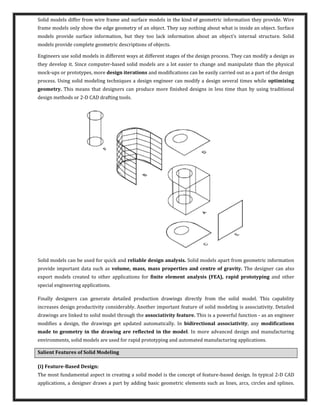
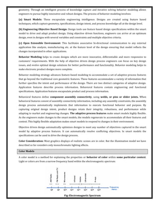
(i)Wire Frame Modeling
In Wire Frame Modeling the object is represented by its edges. In the initial stages of CAD, wire frame models
were in 2-D. Subsequently 3-D wire frame modeling software was introduced. The wire frame model of a box is
shown in Fig. (a). The object appears as if it is made out of thin wires. Fig. (b), (c) and (d) show three objects which
can have the same wire frame model of the box. Thus in the case of complex parts wire frame models can be
confusing. Some clarity can be obtained through hidden line elimination. Though this type of modeling may not
provide unambiguous understanding of the object, this has been the method traditionally used in the 2-D
representation of the object, where orthographic views like plan, elevation, end view etc are used to describe the
object graphically.](https://image.slidesharecdn.com/cadunit-42016-161018092044/85/Surfaces-15-320.jpg)


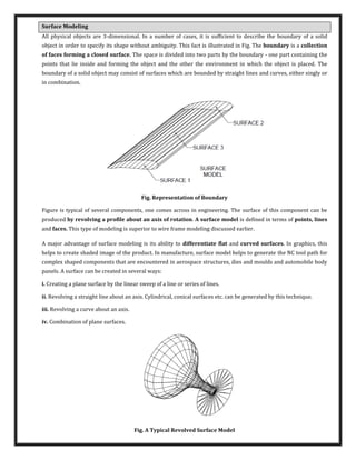
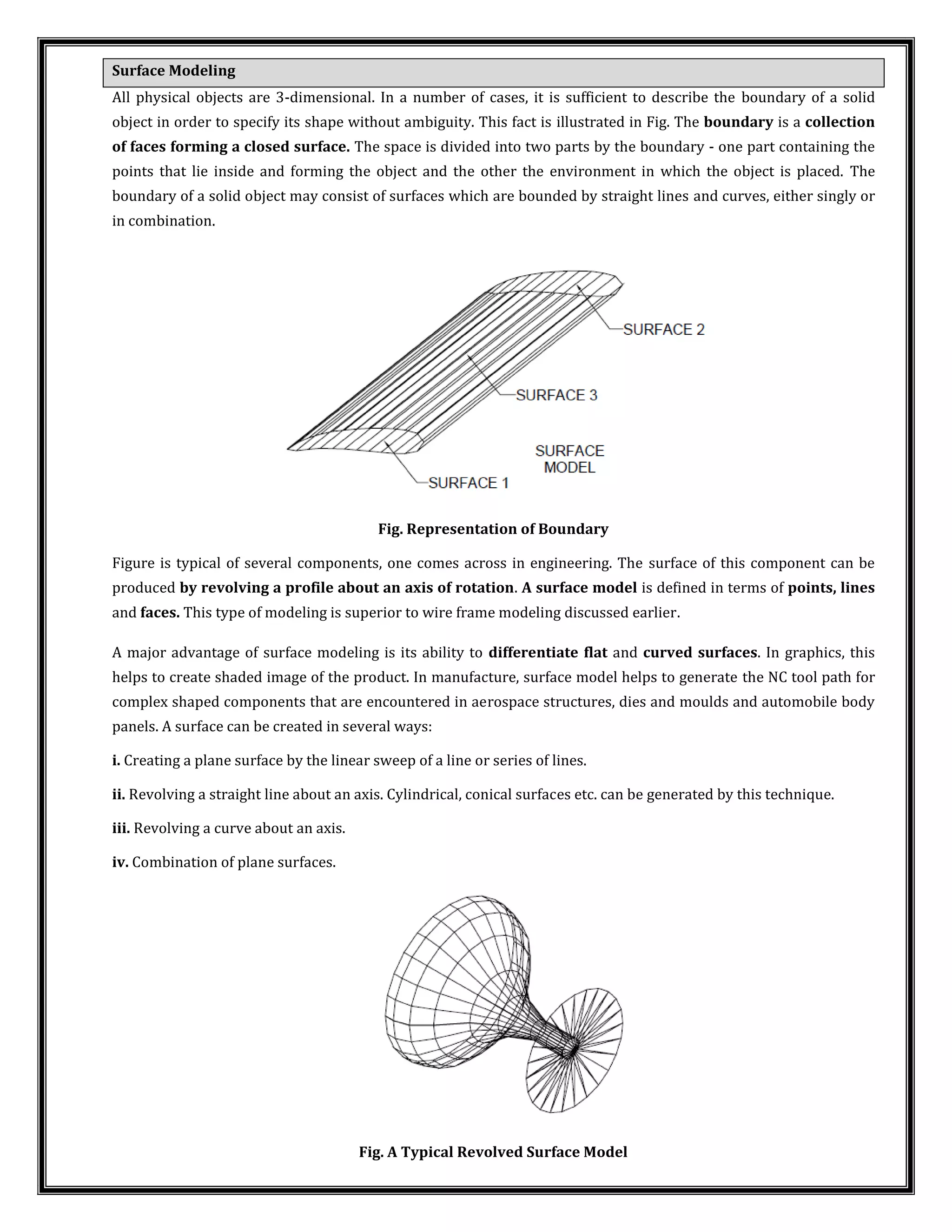
All physical objects have 3D boundaries that define their shape. Surface modeling uses points, lines, and faces to define these boundaries mathematically. There are several types of surfaces, including plane, ruled, revolved, and freeform surfaces. Revolved surfaces are created by rotating a profile around an axis, generating surfaces like cylinders and cones. Curves and surfaces are essential for modeling complex shapes encountered in engineering designs.