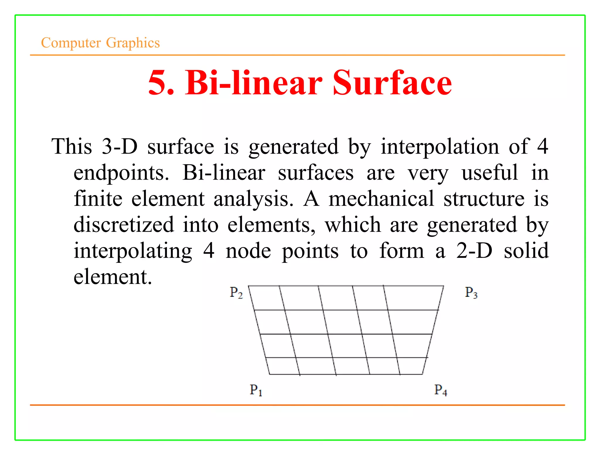
This document discusses different types of surface models used in computer graphics, including: - Plane, ruled, surface of revolution, tabulated, bilinear, Coons patch, and bicubic surfaces. Plane and ruled surfaces are linear, while surfaces of revolution and tabulated surfaces are axisymmetric. Bilinear surfaces are generated by interpolating 4 endpoints and are useful for finite element analysis. Coons patches interpolate 4 edge curves. Bicubic surfaces use parametric curves and interpolation of control points to define smooth surfaces.

1. Computer Graphics
Surface Models
• A surface of an object is more complete and less
ambiguous representation than its wire frame model; it is
an extension of a wire frame model with additional
information.
• A wire frame model can be extracted from a surface model
by deleting all surface entities (not the wireframe entities –
point, lines, or curves!). Databases of surface models are
centralized and associative, manipulation of surface
entities in one view is automatically reflected in the other
views. Surface models can be shaded and represented with
hidden lines.

2. Computer Graphics
Types of Surfaces
1. Plane Surface
• This is the simplest surface, requires 3 non-coincidental points
to define an infinite plane. The plane surface can be used to
generate cross sectional views by intersecting a surface or
solidmodel with it.

3. Computer Graphics
2. Ruled (lofted) Surface
This is a linear surface. It interpolates linearly between
two boundary curves that define the surface.
Boundary curves can be any wire frame entity. The
surface is ideal to represent surfaces that do not have
any twists or kinks.

4. Computer Graphics
3.Surface of Revolution
• This is an axisymmetric surface that can model
axisymmetric objects. It is generated by rotating a
planar wire frame entity in space about the axis of
symmetry of a given angle.

5. Computer Graphics
4.Tabulated Surface
This is a surface generated by translating a
planar curve a given distance along a
specified direction. The plane of the curve
is perpendicular to the axis of the generated
cylinder.

6. Computer Graphics
5. Bi-linear Surface
This 3-D surface is generated by interpolation of 4
endpoints. Bi-linear surfaces are very useful in
finite element analysis. A mechanical structure is
discretized into elements, which are generated by
interpolating 4 node points to form a 2-D solid
element.

7. Computer Graphics
6.Coons Patch
• Coons patch or surface is generated by the
interpolation of 4 edge curves as shown.

8. Computer Graphics
Bi-cubic patches (Surfaces)
• The concept of parametric curves can be
extended to surfaces
• The cubic parametric curve is in the form of
Q(t)=tTM q where q=(q1,q2,q3,q4) : qi control
points, M is the basis matrix (Hermite or
Bezier,…), tT=(t3, t2, t, 1)

9. Computer Graphics
• Now we assume qi to vary along a parameter s,
• Qi(s,t)=tTM [q1(s),q2(s),q3(s),q4(s)]
• qi(s) are themselves cubic curves, we can write
them in the form …

10. Computer Graphics
Bicubic patches
s
M
M
t
M
s
M
s
M
t
t
s
Q
T
T
T
T
T
.
.
.
.
])
[
.
.
],...,
[
.
.
.(
.
)
,
( 4
4
4
41
1
1
1
1
q
q
,
q
,
q
,
q
q
,
q
,
q
,
q 4
3
2
4
3
2
1


where q is a 4x4 matrix
Each column contains the control points of
q1(s),…,q4(s)
x,y,z computed by












44
34
24
14
43
33
23
13
42
32
22
12
41
31
21
11
q
q
q
q
q
q
q
q
q
q
q
q
q
q
q
q
s
M
M
t
t
s
z
s
M
M
t
t
s
y
s
M
M
t
t
s
x
T
z
T
T
y
T
T
x
T
.
.
.
.
)
,
(
.
.
.
.
)
,
(
.
.
.
.
)
,
(
q
q
q




11. Computer Graphics
14/10/2008 Lecture 6 11
Bézier example
• We compute (x,y,z) by
coords
z
of
array
is
q
s
M
q
M
t
t
s
z
coords
y
of
array
is
q
s
M
q
M
t
t
s
y
coords
x
of
array
is
q
s
M
q
M
t
t
s
x
z
T
B
z
B
T
y
T
B
y
B
T
x
T
B
x
B
T
4
4
.
.
.
.
)
,
(
4
4
.
.
.
.
)
,
(
4
4
.
.
.
.
)
,
(







12. Computer Graphics
14/10/2008 Lecture 6 12
Continuity of Bicubic patches.
• Hermite and Bézier patches
– C0 continuity by sharing 4
control points between
patches.
– C1 continuity when both sets
of control points either side of
the edge are collinear with the
edge.