

Recommended
More Related Content
What's hot
What's hot (20)
Similar to Curves wire frame modelling
Similar to Curves wire frame modelling (20)
More from jntuhcej
More from jntuhcej (20)
Recently uploaded
Recently uploaded (20)
Curves wire frame modelling
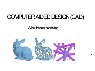
- 2. Wire frame modelling 1. A wire frame model consists of points and curves only. 2. A wire frame model consists of 2 tables the vertex table and edge table. 3. A wire frame model does not face information. 4. Example : Representing a cube defined by 8 vertices and 12 edges
- 3. Advantages & Dis-advantages of wire frame modelling Curves plays important role in generating a wire frame modelling Advantages : 1. Ease of creation. 2. Low level of hardware and software requirements. 3. Data storage requirement is low. Dis-advantages: 1. It can very confusing to visualise. example : A blind hole in a box may be look like a solid cylinder
- 4. Classification of wire frame entities Curves are classified as 1. Analytical curves: • This types of curve can be represented by a simple mathematical equation such as circle or an line • It has a fixed form & cannot be modified to achieve a shape that violates the mathematical equations • The analytical curves are : 1. line 2. arc 3. circle 4. ellipse 5. parabola 6. Hyperbola 2.Synthetic curves: • An interpolated curve is drawn by interpolating the given data points and has a fixed form, dictated by the given data points. • These curves have some limited flexibility in shape creation, dictated by the given data points. The synthetic curves are: 1. Hermite cubic spine or parametric cubic curve or cubic spline. 2. Bezier. 3. B- spline.
- 5. Curves representation methods The mathematical representation of a curves can be classified as: 1. Non- parametric • Explicit • Implicit 2. Parametric Non- Parametric Representation: a) The explicit non- parametric equation is given by : Y = C1+C2X+C3X2+C4X3 • In this equation , there is a unique single value of the dependent variable for each value of the independent variable. b) The implicit non-parametric equation is: (X-XC)2 + (Y-YC)2 = r2 • In this equation , no difference is made between the dependent & the independent variable. Limitations of non-parametric representation are: 1. Explicit non- parametric representation is based on one – to- mapping. 2. This cannot be used for representation of closed curves such as circle or multi- valued curves such as parabola. 3. If the gradient or slope of the curve at a point is vertical , its value is infinity, which cannot be incorporated in the computer programming.
- 6. Representation of curves Types of Curve Equations • Explicit (non-parametric) Y = f(X), Z = g(X) • • Implicit (non-parametric) f(X,Y,Z) = 0 • Parametric X = X(t), Y = Y(t), Z =Z(t)
- 7. Parametric representation of Analytic curves 1. Line A line is defining by connecting two points P1 & P2 . A parameter u is defined such that it has the values 0 & 1 at P1 & P2 respectively. the equation of line is given by: P= P1 + u ( P1 - P2 ) 0 ≤ u ≤1 The length of the line is given by : L the unit vector is given by : n = P2-P1/2
- 8. 2.Circle • A circle with centre (XC , YC) & radius r has an equation as follows: (X-XC)2 + (Y-YC)2 = r2 • If the centre is the origin , the above equation is simplified to : X2 + Y2 = r2 • From the above equation referred to as the non- parametric (implicit) form of the circle. Parametric form of circle is: X = xc+ r cos u Y = yc + r sin u 0 ≤ u ≤1 Z = Zc
- 10. Interpolating and approximating curve: Convex hull The convex hull property ensures that a parametric curve will never pass outside of the convex hull formed by the four control vertices. Convex hull
- 11. Basic Concepts : C 2 C 0 - Zero-order parametric continuity - the two curves sections must have the same coordinate position at the boundary point. C 1 - First-order parametric continuity - tangent lines of the coordinate functions for two successive curve sections are equal at their joining point. C 2 - second-order parametric continuity - both the first and second parametric derivativesof the two curve sections are the same at the intersection,
- 13. Curvature continuity C 0 Continuity : • Consider The end Point of curve f(b) & the start point of the curve g(m) . • If f(b) & g(m) are equal as shown , we shall say curves are C 0 continuous at f(b) = g (m). C 1 Continuity : Two curves are C 1 Continuous at the joining point if the first derivative does not change when crossing one to the other. C 2 Continuity : Two curves are C 2 Continuous at the joining point if in addition to the first derivative , the second derivative is also same when one curve is crossed to the other.
- 14. Hermite cubic Curve • Hermite curves are designed by using two control points and tangent segments at each control point
- 17. Hermite curve in vector form
- 18. where [MH] is the Hermite matrix and V is the geometry (or boundary conditions) vector.
- 19. Properties: •The Hermite curve is composed of a linear combinations of tangents and locations (for each u) •Alternatively, the curve is a linear combination of Hermite basis functions (the matrix M) • The piecewise interpolation scheme is C1 continuous •The blending functions have local support; changing a control point or a tangent vector, changes its local neighbourhood while leaving the rest unchanged Disadvantages: Requires the specification of the tangents. This information is not always available. Limited to 3rd degree polynomial therefore the curve is quite stiff .
- 20. 2.Bezier Curve: • A Bezier Curve is obtained by a defining polygon. • First and last points on the curve are coincident with the first and last points of the polygon. • Degree of polynomial is one less than the number of points • Tangent vectors at the ends of the curve have the same directions as the respective spans • The curve is contained within the convex hull of the defining polygon.
- 22. Properties Beziercurve • TheBezier curve starts at P0and ends at Pn;this is known as‘endpoint interpolation’ property. • TheBezier curve is astraight line when all the control points of acure are collinear. • Thebeginning of the Bezier curve is tangent to the first portion of the Bezier polygon. • ABezier curve canbe divided at any point into two sub curves, each of whichis also aBezier curve. • Afew curves that look like simple, suchasthe circle, cannot be expressed accurately by aBezier; via four piece cubic Bezier curve cansimilar acircle, with amaximum radial error of lessthan one part in athousand(Fig.1). Fig1. Crcular Bezier curve
- 23. • Eachquadratic Bezier curve is become acubic Bezier curve, and more commonly, each degree ‘n’ Bezier curve is also adegree ‘m’ curve for any m >n. • Bezier curves have the different diminishing property. ABezier curves does not ‘ripple’ more than the polygon of its control points, and may actually ‘ripple’ less than that. • Bezier curve is similar with respect to t and (1-t). This represents that the sequence of control points defining the curve canbe changeswithout modify ofthe curve shape. • Bezier curve shape can be edited by either modifying one or more vertices of its polygon or by keeping the polygon unchanged or simplifying multiple coincident points at avertex (Fig.2). Fig: 2. Bezier curve shpe
- 25. 3.B-spline Curve Ni,k(u)'s are B-spline basis functions of degree p. • Theform of aB-spline curve is very similar to that of aBézier curve. Unlike aBézier curve, aB-spline curve involves more information, namely: aset of n+1 control points, a knot vector of m+1 knots, and adegreep. • Given n +1 control points P0, P1, ..., Pn and aknot vector U={ u0, u1, ..., um }, the B- spline curve of degree p defined by these control points and knotvector. • Theknot points divide aB-spline curve into curve segments, each of which is defined on aknot span. m =n +p + 1. • Itprovide local control of the curve shape. • It also provide the ability to add control points without increasing the degree of the curve. • B-spline curves have the ability to interpolate or approximate aset ofgiven data points. The B-spline curve defined by n+1 control points Pi is given by
- 26. • Thedegree of aBézier basis function depends on the number of controlpoints. • Tochangethe shapeof aB-spline curve, one canmodify one or more of these control parameters: the positions of control points, the positions of knots, and the degree of the curve. • If the knot vector does not have any particular structure, the generated curve will not touch the first and last legsof the control polyline asshown in the left figure below. • Thistype of B-spline curves is called open B-splinecurves. Properties of B-SplineCurve:
- 27. The first property ensures that the relationship between the curve and its defining control points is invariant under affinetransformations. The second property guarantees that the curve segment lies completely within the convex hull of Pi. The third property indicates that each segment of a B-spline curve is influenced by only k control points or eachcontrol point affects only only k curve segments, as shown in Figure 1. It is useful to notice that the Bernstein polynomial, has the same first two properties mentionedabove.
- 28. TheB-spline function TheB-spline function also hasthe property of recursion,which is definedas