Downloaded 426 times
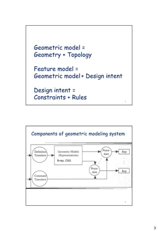

![16
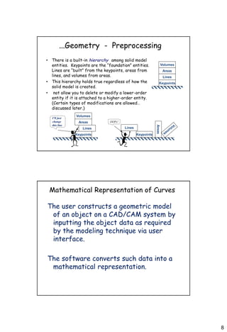
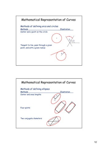
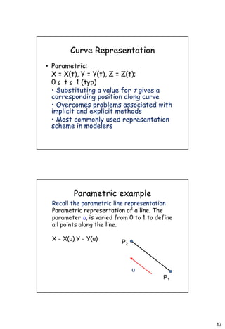
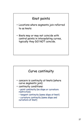
Curve Representation
• Curves may be defined using different
equation formats.
• explicit Y = f(X), Z = g(X)
• implicit f(X,Y,Z) = 0
• parametric X = X(t), Y = Y(t), Z = Z(t)
• The explicit and implicit formats have
serious disadvantages for use in
computer-based modeling
Parametric form
• Equations are de-coupled
• x = f (u)
• Matrix form: p (u) = [ u3 u2 u 1 ]
[ A ]](https://image.slidesharecdn.com/geometricmodelcurve-150820094100-lva1-app6891/85/Geometric-model-curve-16-320.jpg)
![18
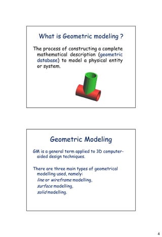
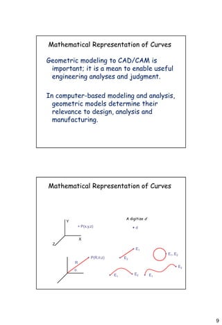
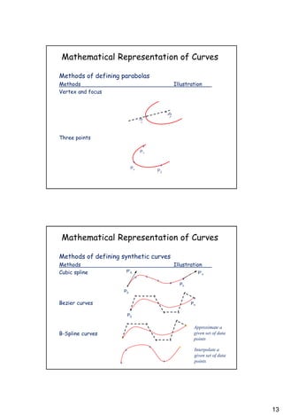
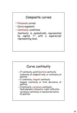
Parametric Line
• Line defined in terms of its endpoints
• Positions along the line are based upon
the parameter value
– For example, the midpoint of a line occurs at u
= 0.5
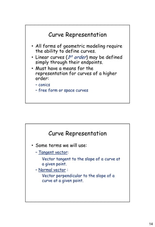
Parametric Line
• This means a parametric line can be defined
by:
L(u) = [x(u), y(u), z(u)] = A + (B - A)u
where A and B and the line endpoints. e.g. A
line from point A = (2,4,1) to point B = (7,5,5)
can be represented as:
x(u) = 2 + (7-2)u = 2 + 5u
y(u) = 4 + (5-4)u = 4 + u
z(u) = 1 + (5-1)u = 1 + 4u](https://image.slidesharecdn.com/geometricmodelcurve-150820094100-lva1-app6891/85/Geometric-model-curve-18-320.jpg)
![19
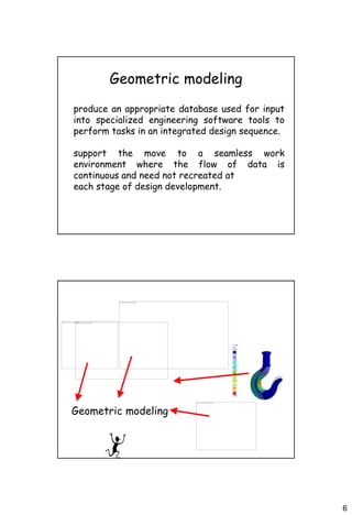
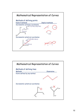
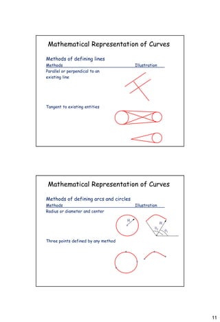
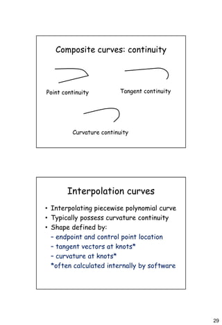
Parametric cubic curves
• Algebraic form
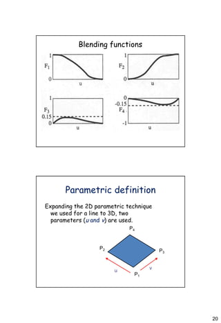
• Geometric form: blending fn *
geometric (boundary) conditions
• Blending function: p (u) = [ F1 F2 F3 F4 ]
[ p(0), p(1), pu(0), pu(1) ]
• Magnitude and direction of tangent
vectors
• Cubic Hermite blending function
Boundary conditions](https://image.slidesharecdn.com/geometricmodelcurve-150820094100-lva1-app6891/85/Geometric-model-curve-19-320.jpg)


This document discusses geometric modeling and curves. It provides information on: - Geometric modeling is the process of creating mathematical models of physical objects and systems using computer software. - There are different types of geometric models including wireframe, surface, and solid modeling. - Curves can be represented mathematically in both implicit and parametric forms, with parametric being most common in modeling as it overcomes limitations of other forms. - Parametric curves define a curve using a parameter, where varying the parameter provides points on the curve. Common parametric representations include lines, conics, and higher-order curves composed of simpler curve segments.