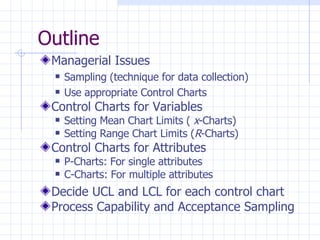
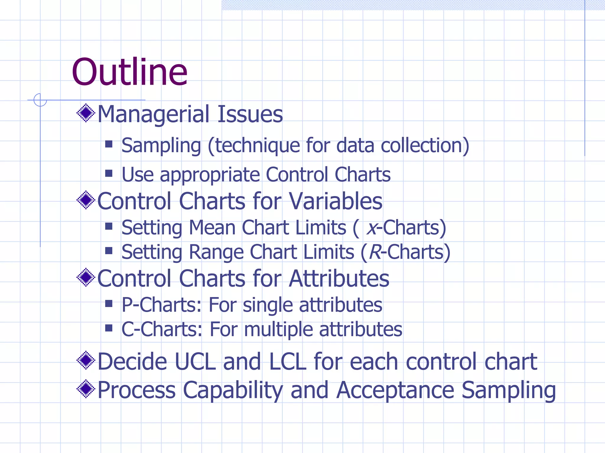
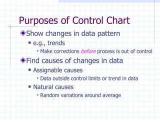
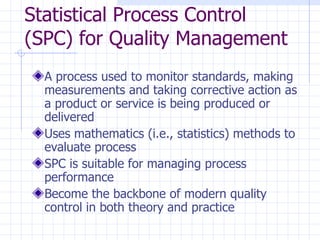
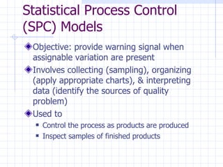
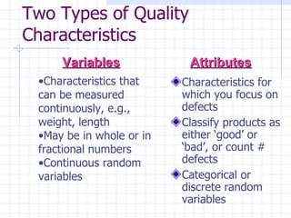
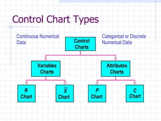
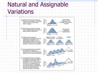
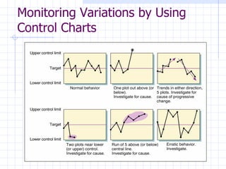
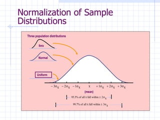
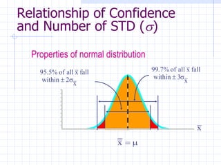
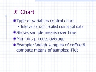
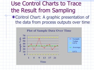
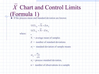
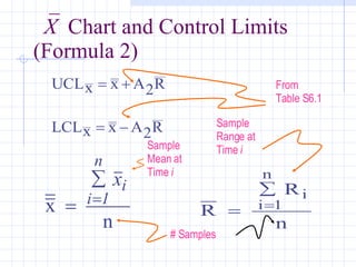
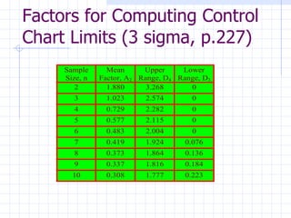
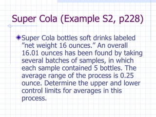
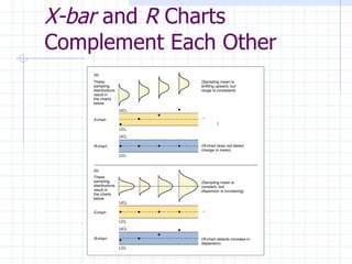
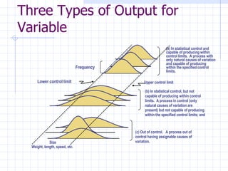
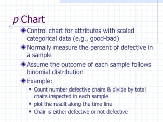
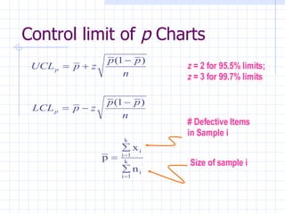
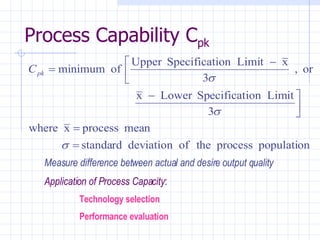
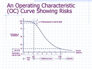
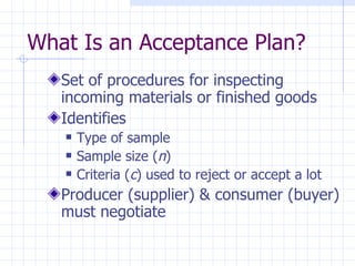
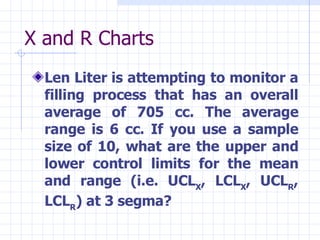
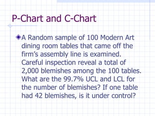
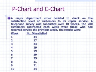
This document discusses statistical process control (SPC) techniques for quality management, including control charts for variables and attributes, sampling methods, process capability analysis, and acceptance sampling. It outlines how to select appropriate control charts, set control limits, identify assignable and natural causes of variation, and use control charts to monitor processes over time for process improvement.

1. Outline Managerial Issues Sampling (technique for data collection) Use appropriate Control Charts Control Charts for Variables Setting Mean Chart Limits ( x -Charts) Setting Range Chart Limits ( R -Charts) Control Charts for Attributes P-Charts: For single attributes C-Charts: For multiple attributes Decide UCL and LCL for each control chart Process Capability and Acceptance Sampling

2. Show changes in data pattern e.g., trends Make corrections before process is out of control Find causes of changes in data Assignable causes Data outside control limits or trend in data Natural causes Random variations around average Purposes of Control Chart

3. Statistical Process Control (SPC) for Quality Management A process used to monitor standards, making measurements and taking corrective action as a product or service is being produced or delivered Uses mathematics (i.e., statistics) methods to evaluate process SPC is suitable for managing process performance Become the backbone of modern quality control in both theory and practice

4. Objective: provide warning signal when assignable variation are present Involves collecting (sampling), organizing (apply appropriate charts), & interpreting data (identify the sources of quality problem) Used to Control the process as products are produced Inspect samples of finished products Statistical Process Control (SPC) Models

5. Natural (Normal) Variations Comprised of a myriad of small sources that are always present in a process and affect all elements of the process. Vibration Humidity Temperature Lighting Other uncontrollable factors Usually is difficult or costly to control

6. Assignable (Abnormal) Variations Caused by the controllable quality problems in a product or process. Poor product design Machines out of order Tools wear out Poor incoming materials Low skills and qualification of workers Workers’ fatigue Unpleasant working conditions Poor training

7. Statistical Process Control Steps Produce Good Provide Service Stop Process Yes No Assign. Variation? Take Sample Inspect Sample Find Out Why Create Control Chart Start

8. Characteristics for which you focus on defects Classify products as either ‘good’ or ‘bad’, or count # defects Categorical or discrete random variables Two Types of Quality Characteristics Attributes Variables Characteristics that can be measured continuously, e.g., weight, length May be in whole or in fractional numbers Continuous random variables

9. Control Chart Types Control Charts R Chart Variables Charts Attributes Charts X Chart P Chart C Chart Continuous Numerical Data Categorical or Discrete Numerical Data

10. Natural and Assignable Variations

11. Monitoring Variations by Using Control Charts

12. Sampling Techniques in Quality Control Why sampling Too costly to inspect all outcomes from a process Sample size: SPC usually uses average of a small number of items as a sample Individual pieces tend to be too erratic to make trends quickly visible Serve as the input of all control charts Both sampling rule and sample sizes affect the cost and accuracy of quality control

13. Monitoring the Weights of Oat Flakes (Example S1, p226) Purpose of sampling and the sampling rule The weights of boxes of Oat Flakes within a large production lot are sampled each hour Sample Frequency Sampling every hour Sample size In each sampling, 9 boxes are randomly selected and weighted Confidence and number of standard deviation  = 2 for 95.5% confidence;  = 3 for 99.73% confidence

14. Theoretical Basis of Sampling As sample size gets large enough, sampling distribution becomes almost normal regardless of population distribution. Central Limit Theorem

15. Central Limit Theorem Mean Standard deviation (STD)

16. Normalization of Sample Distributions Uniform Normal Beta (mean) Three population distributions

17. Relationship of Confidence and Number of STD (  ) Properties of normal distribution

18. Type of variables control chart Interval or ratio scaled numerical data Shows sample means over time Monitors process average Example: Weigh samples of coffee & compute means of samples; Plot  X Chart

19. Use Control Charts to Trace the Result from Sampling Control Chart: A graphic presentation of the data from process outputs over time

20.  X Chart and Control Limits (Formula 1)  If the process mean and standard deviation are known: where: _ X = average mean of samples Z = number of standard deviations  x = standard deviation of sample means  x = process standard deviation, n = number of observations in a sample

21. Sample Range at Time i # Samples Sample Mean at Time i From Table S6.1  X Chart and Control Limits (Formula 2)

22. Factors for Computing Control Chart Limits (3 sigma, p.227)

23. Super Cola (Example S2, p228) Super Cola bottles soft drinks labeled ”net weight 16 ounces.” An overall 16.01 ounces has been found by taking several batches of samples, in which each sample contained 5 bottles. The average range of the process is 0.25 ounce. Determine the upper and lower control limits for averages in this process.

24. Type of variables control chart Interval or ratio scaled numerical data Shows sample ranges over time Difference between smallest & largest values in inspection sample Monitors variability in process Example: Weigh samples of coffee Compute ranges of samples Plot R Chart

25. R Chart Control Limits Sample Range at Time i # Samples From Table S6.1

26. Loading Trucks (Example S3, p228) The average range of a process for loading trucks is 5.3 pounds. If the sample size is 5, determine the upper and lower control limits for the R -Chart.

27. Steps to Follow When Using X-bar or R Control Charts Collect 20 to 25 samples of n=4 or n=5 from a stable process and compute the mean. Compute the overall means, set approximate control limits,and calculate the preliminary upper and lower control limits. Graph the sample means and ranges on their respective control charts and determine whether they fall outside the acceptable limits. Investigate points or patterns that indicate the process is out of control. Assign causes for the variations. Collect additional samples and revalidate the control limits.

28. X-bar and R Charts Complement Each Other

29. Three Types of Output for Variable Frequency Lower control limit Size Weight, length, speed, etc. Upper control limit (b) In statistical control, but not capable of producing within control limits. A process in control (only natural causes of variation are present) but not capable of producing within the specified control limits; and (c) Out of control. A process out of control having assignable causes of variation. (a) In statistical control and capable of producing within control limits. A process with only natural causes of variation and capable of producing within the specified control limits.

30. Control chart for attributes with scaled categorical data (e.g., good-bad) Normally measure the percent of defective in a sample Assume the outcome of each sample follows binomial distribution Example: Count number defective chairs & divide by total chairs inspected in each sample plot the result along the time line Chair is either defective or not defective p Chart

31. Control limit of p Charts # Defective Items in Sample i Size of sample i z = 2 for 95.5% limits; z = 3 for 99.7% limits

32. ARCO (Example S4, p231) Data-entry clerks at ARCO key in thousands of insurance records each day. Samples of the work of 20 clerks are shown in the table. One hundred records by each clerk were carefully examined and the number of errors counted. The fraction in each sample was then computed as p-bar . Set the control limits to include 99.73% of the random variation in the entry process when it is in control.

33. Attributes control chart for discrete data Shows the number of nonconformities (defects) in a unit (unit may be chair, steel sheet, car etc). UCL and LCL are not sensitive to the sample size Assume the defect number is Poison distribution Example: Derive the average number of defects (scratches, chips etc.) in each chair of a sample of 100 chairs Plot the average number along the timeline c - Chart

34. Control Limits of c-Charts # Defects in Unit i # Units Sampled Use 3 for 99.7% limits

35. Red Top Cap (Example S5, p233) Red Top Cab Company receives several complaints per day about the behavior of its drivers. Over a 9-day period (where days are the units of measure), the owner received the following number of calls from rate passengers: {3, 0, 8, 9, 6, 7, 4, 9, 8} for a total of 54 complaints. Compute the UCL and LCL limits at 99.7% confidence.

36. Managerial Issues and Control Charts Three major decisions regarding control chart Select the points in the process that need SPC Which process point is critical Which point tends to be out of control Select appropriate chart and UCL/LCL Set clear and specific SPC policies for workers to follow

37. Process Capability C pk Measure difference between actual and desire output quality Application of Process Capacity : Technology selection Performance evaluation

38. Meanings of C pk Measures C pk = negative number C pk = zero C pk = between 0 and 1 C pk = 1 C pk > 1

39. Form of quality testing used for incoming materials or finished goods e.g., purchased material & components Procedure Take one or more samples at random from a lot (shipment) of items Inspect each of the items in the sample Decide whether to reject the whole lot based on the inspection results What Is Acceptance Sampling?

40. Shows how well a sampling plan discriminates between good & bad lots (shipments) Shows the relationship between the probability of accepting a lot & its quality Operating Characteristics Curve

41. OC Curve 100% Inspection % Defective in Lot P(Accept Whole Shipment) 100% 0% Cut-Off Return whole shipment Keep whole shipment 1 2 3 4 5 6 7 8 9 10 0

42. OC Curve with Less than 100% Sampling P(Accept Whole Shipment) 100% 0% % Defective in Lot Cut-Off Return whole shipment Keep whole shipment Probability is not 100%: Risk of keeping bad shipment or returning good one. 1 2 3 4 5 6 7 8 9 10 0

43. Supplier/Producer's risk (  ) Probability of rejecting a good lot (type I error) Probability that a lot get rejected when fraction defective is AQL Buyer/Consumer's risk (ß) Probability of accepting a bad lot (type II error) Probability of accepting a lot when fraction defective is LTPD Producer’s & Consumer’s Risk

44. Acceptable quality level (AQL) Quality level of a good lot from producer’s standard Producer (supplier) does not want lots with fewer defects than AQL rejected Lot tolerance percent defective (LTPD) Quality level of a bad lot from buyer’s standard Consumer (buyer) does not want lots with more defects than LTPD accepted AQL & LTPD

45. An Operating Characteristic (OC) Curve Showing Risks  = 0.10 Consumer’s risk for LTPD Probability of Acceptance Percent Defective 0 1 2 3 4 5 6 7 8 100 95 75 50 25 10 0  = 0.05 producer’s risk for AQL Bad lots Indifference zone Good lots LTPD AQL

46. Set of procedures for inspecting incoming materials or finished goods Identifies Type of sample Sample size ( n ) Criteria ( c ) used to reject or accept a lot Producer (supplier) & consumer (buyer) must negotiate What Is an Acceptance Plan?

47. Assignment #3 Solve and Answer the following problems in the textbook (p245 to p249) S6.6, S6.8 (x-Chart and R-Chart) S.6.15, S6.16, S6.17, S6.18 (P-Chart) S6.21, S6.23, S6.24 (C-Chart) S6.29, S6.30, S6.31 (process capability)

48. X and R Charts Len Liter is attempting to monitor a filling process that has an overall average of 705 cc. The average range is 6 cc. If you use a sample size of 10, what are the upper and lower control limits for the mean and range (i.e. UCL X , LCL X , UCL R , LCL R ) at 3 segma?

49. P-Chart and C-Chart A Random sample of 100 Modern Art dining room tables that came off the firm’s assembly line is examined. Careful inspection reveal a total of 2,000 blemishes among the 100 tables. What are the 99.7% UCL and LCL for the number of blemishes? If one table had 42 blemishes, is it under control?

50. P-Chart and C-Chart A major department store decided to check on the satisfaction level of customers to its repair service. A telephone survey was conducted over 10 weeks. The 200 customers contracted each week were those who had received service the previous week. The results were: Week No. Dissatisfied 1 44 2 27 3 34 4 29 5 19 6 39 7 25 8 31 9 21 10 34