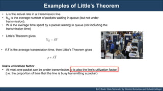
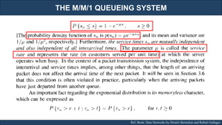
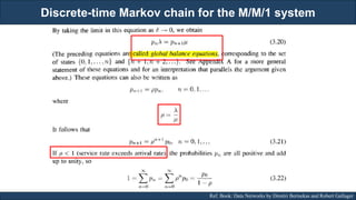
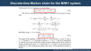
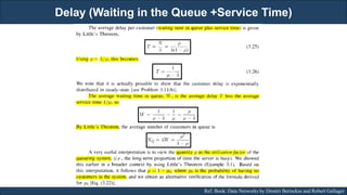
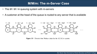
Downloaded 33 times


![Poisson Process and their Properties
RJEs: Remote job entry points
27
Ref. Book - Introduction to Probability by Dimitri P. Bertsekas and John N. Tsitsiklis
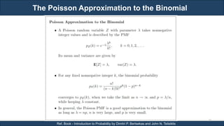
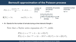
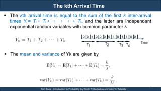
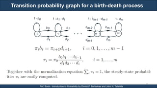
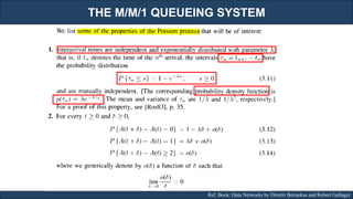
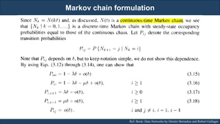
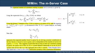
The first property states that arrivals are “equally likely” at all times. The arrivals during any time
interval of length τ are statistically the same, in the sense that they obey the same probability law.
This is a counterpart of the assumption that the success probability p in a Bernoulli process is
constant over time.
To interpret the second property, consider a particular interval [t, t], of length t − t. The unconditional
probability of k arrivals during that interval is P(k, t − t). Suppose now that we are given complete or
partial information on the arrivals outside this interval. Property (b) states that this information is
irrelevant: the conditional probability of k arrivals during [t, t] remains equal to the unconditional
probability P(k, t − t). This property is analogous to the independence of trials in a Bernoulli process.
The third property is critical. The o(τ ) and o1(τ ) terms are meant to be negligible in comparison to τ
, when the interval length τ is very small. They can be thought of as the O(τ 2) terms in a Taylor
series expansion of P(k, τ). Thus, for small τ , the probability of a single arrival is roughly λτ, plus a
negligible term. Similarly, for small τ , the probability of zero arrivals is roughly 1 − λτ. Note that the
probability of two or more arrivals is](https://image.slidesharecdn.com/stochasticprocessanditsapplications-final-231208224707-f76b35c6/85/Stochastic-Process-and-its-Applications-27-320.jpg)

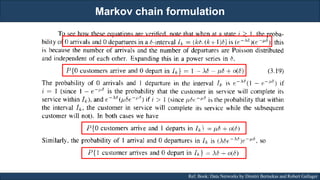
![Bernoulli approximation of the Poisson process
RJEs: Remote job entry points
30
Ref. Book - Introduction to Probability by Dimitri P. Bertsekas and John N. Tsitsiklis
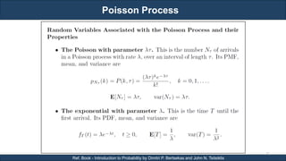
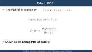
Let us now derive the probability law for the time T of the first arrival, assuming that the process
starts at time zero.
Note that we have T > t if and only if there are no arrivals during the interval [0, t]. Therefore
We then differentiate the CDF FT (t) of T, and obtain the PDF formula](https://image.slidesharecdn.com/stochasticprocessanditsapplications-final-231208224707-f76b35c6/85/Stochastic-Process-and-its-Applications-30-320.jpg)


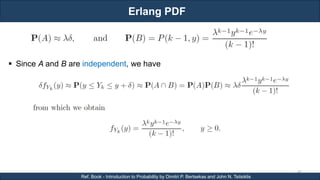
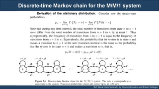
![Erlang PDF
RJEs: Remote job entry points
39
Ref. Book - Introduction to Probability by Dimitri P. Bertsekas and John N. Tsitsiklis
For a small δ, the product is the probability that the kth arrival occurs between times y
and y+δ.
When δ is very small, the probability of more than one arrival during the interval [y, y + δ] is
negligible.
Thus, the kth arrival occurs between y and y + δ if and only if the following two events A and B
occur:
(a) event A: there is an arrival during the interval [y, y + δ];
(b) event B: there are exactly k − 1 arrivals before time y.
The probabilities of these two events are](https://image.slidesharecdn.com/stochasticprocessanditsapplications-final-231208224707-f76b35c6/85/Stochastic-Process-and-its-Applications-39-320.jpg)


The document discusses stochastic processes and provides examples of different types of stochastic processes including Bernoulli processes and Poisson processes. It covers key concepts such as arrival-type processes, Markov processes, discrete and continuous time Markov chains, and simulating different stochastic processes. It also discusses statistics methods like MLE, MAP, and Bayesian estimation that are relevant to stochastic processes. Reference books and materials on the topic are provided.