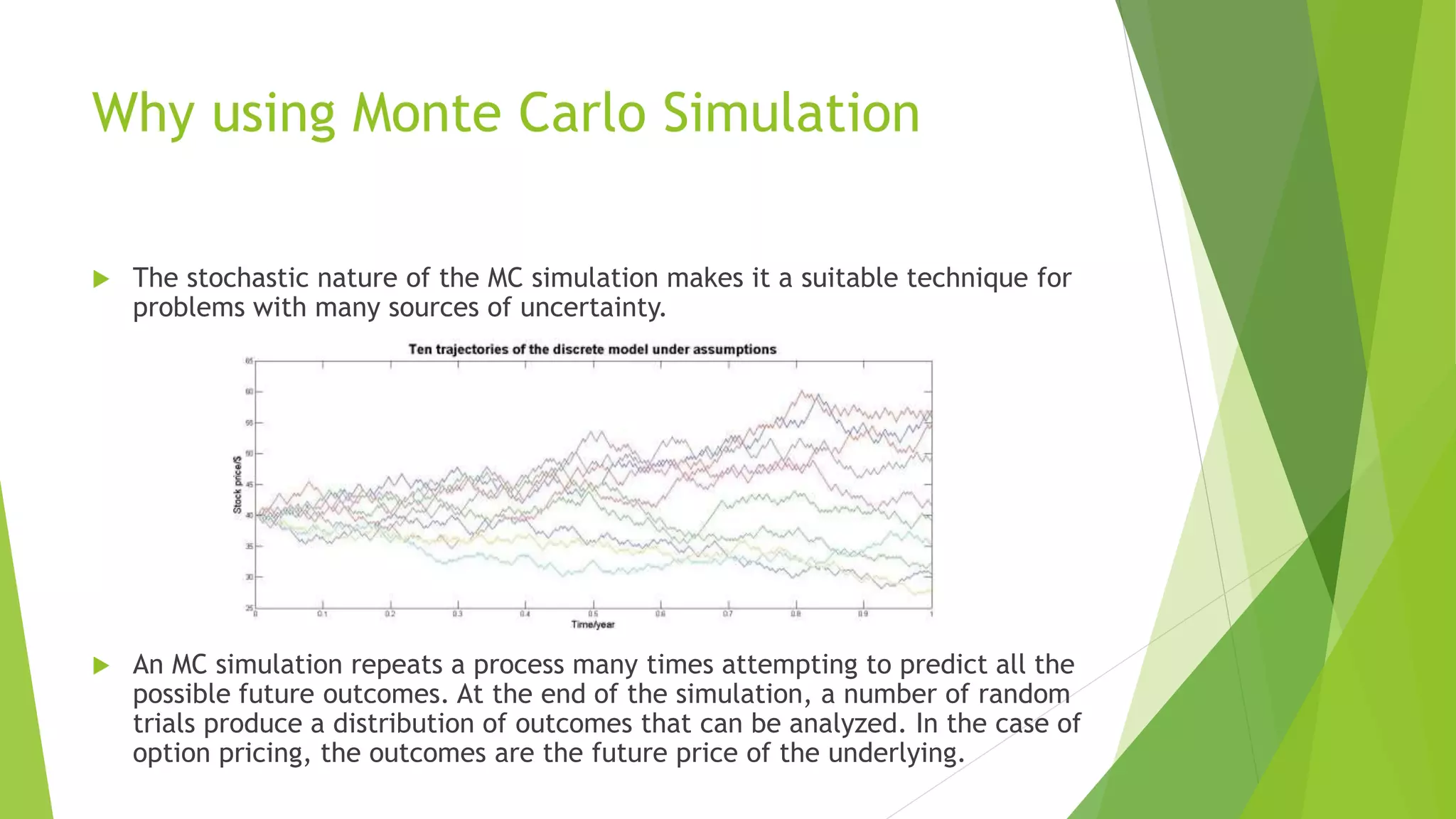
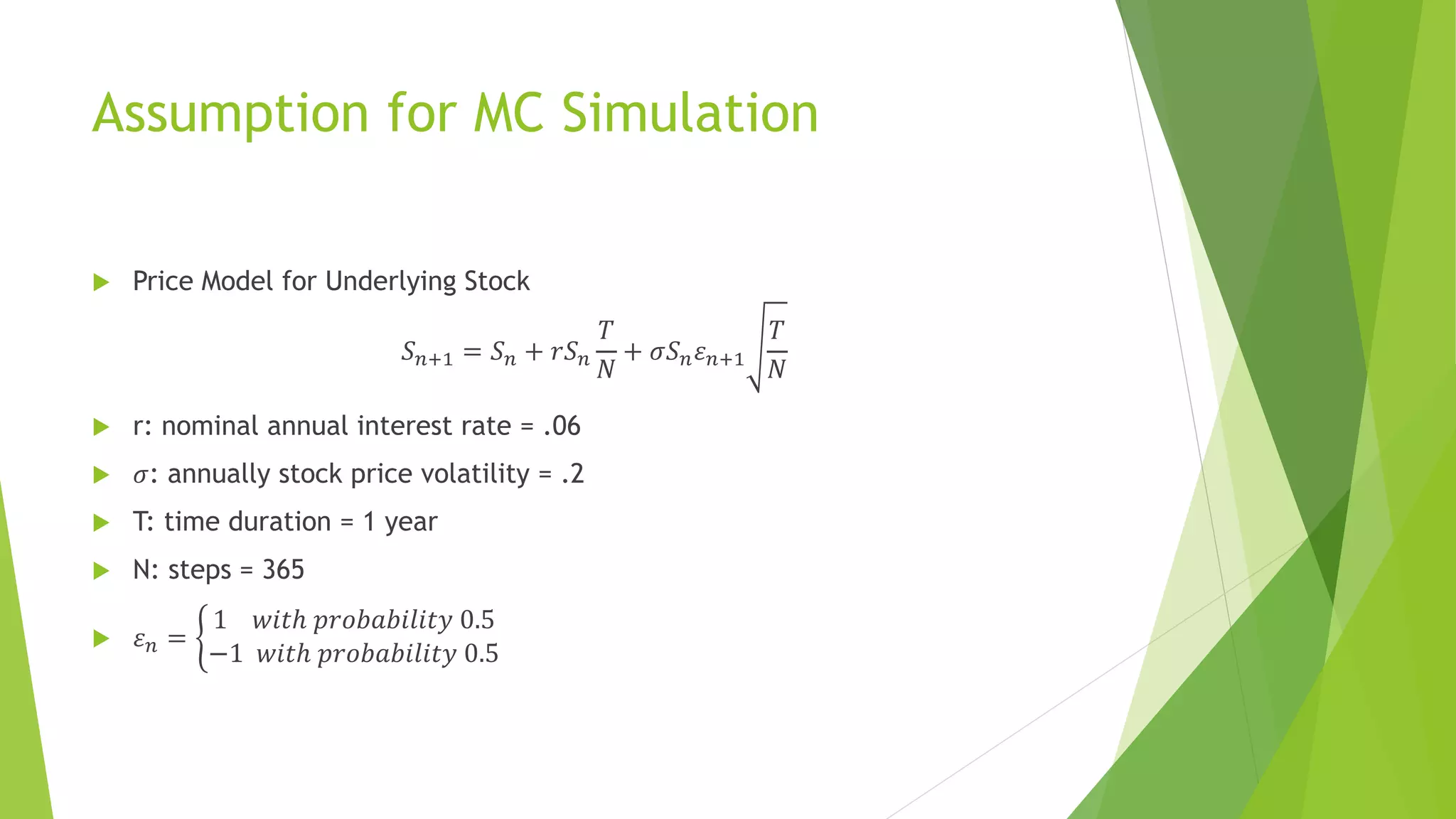
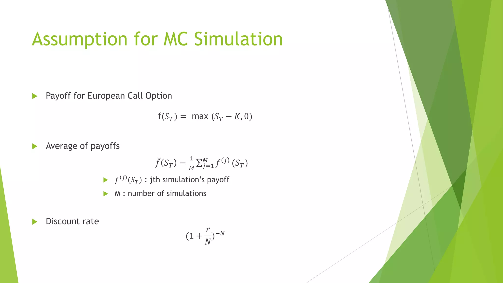
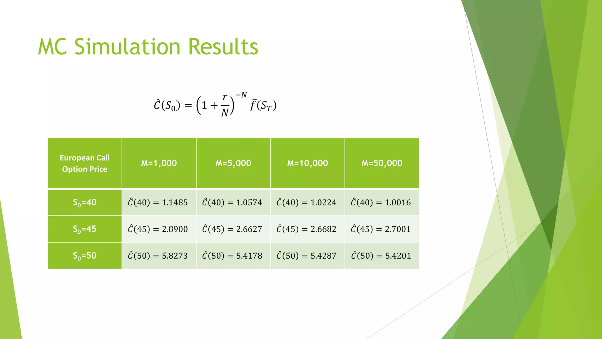
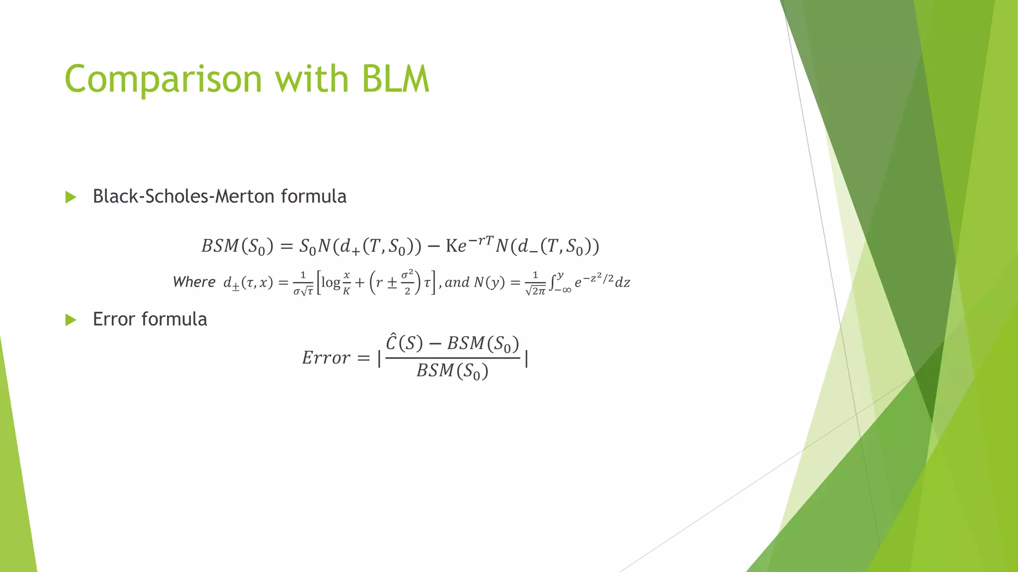
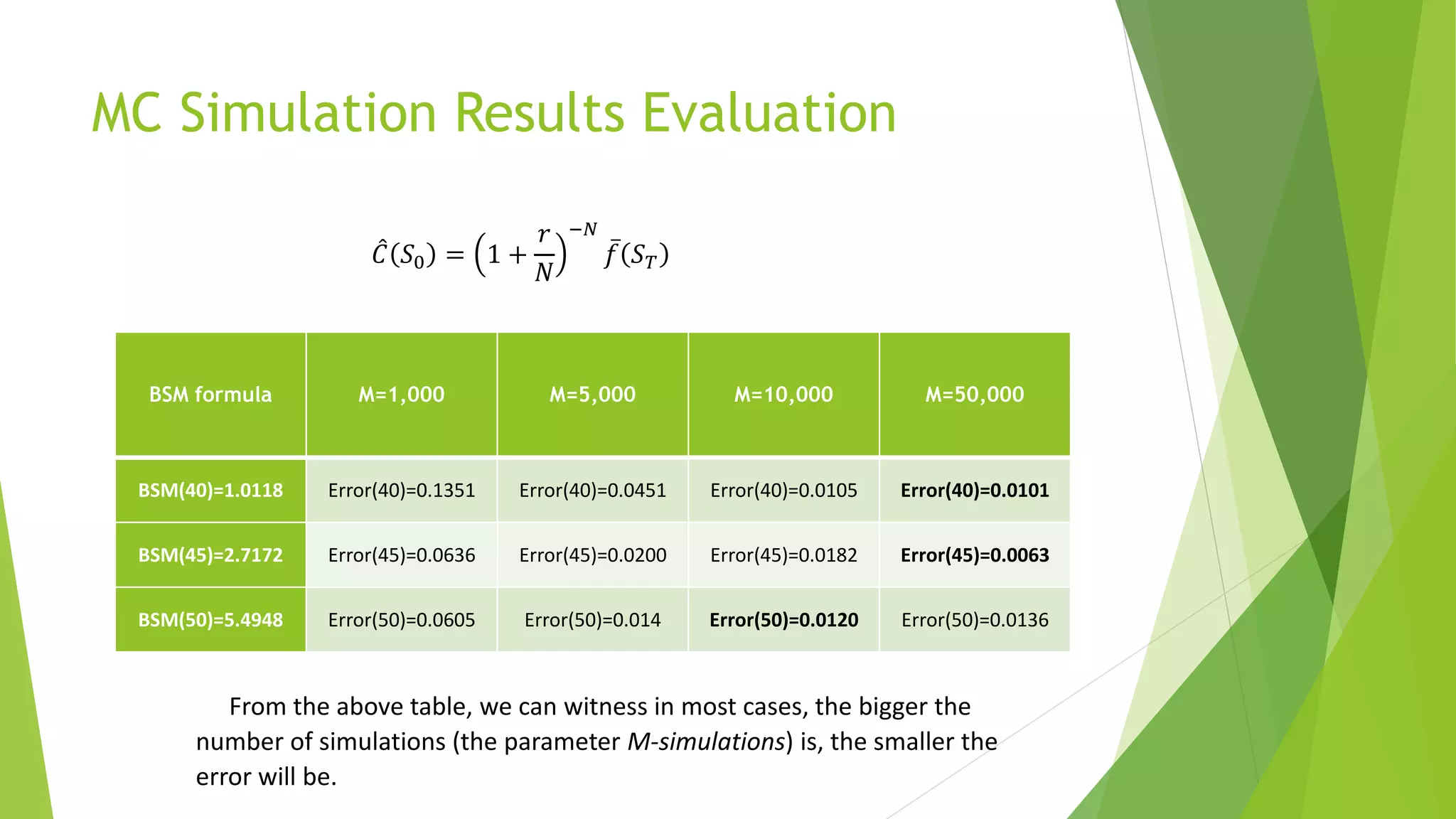
in European Call Option Pricing
Yingzhou HE/ Yuchen DUAN
CONTENT
 REASON
 PROCEDURE
 ASSUMPTION
 RESULT
 EVALUATION
Why using Monte Carlo Simulation
 Options
 Stock option
 Bond option
 index option
 Future option
 Currency option
 …
 Uncertainty
 Stock price
 Annualized interest rate
 Stock index
 futures price
 Underlying currency price & exchange rate
 …
OPTION PRICE IS DIFFICULT TO CALCULATE
DUE TO MULTIPLE SOURCES OF UNCERTAINTY
Why using Monte Carlo Simulation
 The stochastic nature of the MC simulation makes it a suitable technique for
problems with many sources of uncertainty.
 An MC simulation repeats a process many times attempting to predict all the
possible future outcomes. At the end of the simulation, a number of random
trials produce a distribution of outcomes that can be analyzed. In the case of
option pricing, the outcomes are the future price of the underlying.
MC Simulation Option Price Procedure
 Step1: generate a large number of possible (but random) price paths for
the underlying via simulation
 Step2: calculate the associated payoff of the option for each path
 Step3: average the payoffs
 Step4: discount to today
Assumption for MC Simulation
 Price Model for Underlying Stock
𝑆 𝑛+1 = 𝑆 𝑛 + 𝑟𝑆 𝑛
𝑇
𝑁
+ 𝜎𝑆 𝑛 𝜀 𝑛+1
𝑇
𝑁
 r: nominal annual interest rate = .06
 𝜎: annually stock price volatility = .2
 T: time duration = 1 year
 N: steps = 365
 𝜀 𝑛 =
1 𝑤𝑖𝑡ℎ 𝑝𝑟𝑜𝑏𝑎𝑏𝑖𝑙𝑖𝑡𝑦 0.5
−1 𝑤𝑖𝑡ℎ 𝑝𝑟𝑜𝑏𝑎𝑏𝑖𝑙𝑖𝑡𝑦 0.5
Assumption for MC Simulation
 Payoff for European Call Option
f(𝑆 𝑇) = max (𝑆 𝑇 − 𝐾, 0)
 Average of payoffs
𝑓 𝑆 𝑇 =
1
𝑀 𝑗=1
𝑀
𝑓 𝑗
(𝑆 𝑇)
 𝑓 𝑗
(𝑆 𝑇) : jth simulation’s payoff
 M : number of simulations
 Discount rate
(1 +
𝑟
𝑁
)−𝑁
MC Simulation Results
European Call
Option Price
M=1,000 M=5,000 M=10,000 M=50,000
S0=40 𝐶 40 = 1.1485 𝐶 40 = 1.0574 𝐶 40 = 1.0224 𝐶 40 = 1.0016
S0=45 𝐶 45 = 2.8900 𝐶 45 = 2.6627 𝐶 45 = 2.6682 𝐶 45 = 2.7001
S0=50 𝐶 50 = 5.8273 𝐶 50 = 5.4178 𝐶 50 = 5.4287 𝐶 50 = 5.4201
𝐶 𝑆0 = 1 +
𝑟
𝑁
−𝑁
𝑓 𝑆 𝑇
Comparison with BLM
 Black-Scholes-Merton formula
𝐵𝑆𝑀 𝑆0 = 𝑆0 𝑁(𝑑+ 𝑇, 𝑆0 ) − K𝑒−𝑟𝑇
𝑁(𝑑− 𝑇, 𝑆0 )
Where 𝑑± 𝜏, 𝑥 =
1
𝜎 𝜏
log
𝑥
𝐾
+ 𝑟 ±
𝜎2
2
𝜏 , 𝑎𝑛𝑑 𝑁 𝑦 =
1
2𝜋 −∞
𝑦
𝑒−𝑧2/2
𝑑𝑧
 Error formula
𝐸𝑟𝑟𝑜𝑟 = |
𝐶 𝑆 − 𝐵𝑆𝑀(𝑆0)
𝐵𝑆𝑀(𝑆0)
|
MC Simulation Results Evaluation
BSM formula M=1,000 M=5,000 M=10,000 M=50,000
BSM(40)=1.0118 Error(40)=0.1351 Error(40)=0.0451 Error(40)=0.0105 Error(40)=0.0101
BSM(45)=2.7172 Error(45)=0.0636 Error(45)=0.0200 Error(45)=0.0182 Error(45)=0.0063
BSM(50)=5.4948 Error(50)=0.0605 Error(50)=0.014 Error(50)=0.0120 Error(50)=0.0136
𝐶 𝑆0 = 1 +
𝑟
𝑁
−𝑁
𝑓 𝑆 𝑇
From the above table, we can witness in most cases, the bigger the
number of simulations (the parameter M-simulations) is, the smaller the
error will be.

Monte carlo simulation

  • 1.
    in European CallOption Pricing Yingzhou HE/ Yuchen DUAN
  • 2.
    CONTENT  REASON  PROCEDURE ASSUMPTION  RESULT  EVALUATION
  • 3.
    Why using MonteCarlo Simulation  Options  Stock option  Bond option  index option  Future option  Currency option  …  Uncertainty  Stock price  Annualized interest rate  Stock index  futures price  Underlying currency price & exchange rate  … OPTION PRICE IS DIFFICULT TO CALCULATE DUE TO MULTIPLE SOURCES OF UNCERTAINTY
  • 4.
    Why using MonteCarlo Simulation  The stochastic nature of the MC simulation makes it a suitable technique for problems with many sources of uncertainty.  An MC simulation repeats a process many times attempting to predict all the possible future outcomes. At the end of the simulation, a number of random trials produce a distribution of outcomes that can be analyzed. In the case of option pricing, the outcomes are the future price of the underlying.
  • 5.
    MC Simulation OptionPrice Procedure  Step1: generate a large number of possible (but random) price paths for the underlying via simulation  Step2: calculate the associated payoff of the option for each path  Step3: average the payoffs  Step4: discount to today
  • 6.
    Assumption for MCSimulation  Price Model for Underlying Stock 𝑆 𝑛+1 = 𝑆 𝑛 + 𝑟𝑆 𝑛 𝑇 𝑁 + 𝜎𝑆 𝑛 𝜀 𝑛+1 𝑇 𝑁  r: nominal annual interest rate = .06  𝜎: annually stock price volatility = .2  T: time duration = 1 year  N: steps = 365  𝜀 𝑛 = 1 𝑤𝑖𝑡ℎ 𝑝𝑟𝑜𝑏𝑎𝑏𝑖𝑙𝑖𝑡𝑦 0.5 −1 𝑤𝑖𝑡ℎ 𝑝𝑟𝑜𝑏𝑎𝑏𝑖𝑙𝑖𝑡𝑦 0.5
  • 7.
    Assumption for MCSimulation  Payoff for European Call Option f(𝑆 𝑇) = max (𝑆 𝑇 − 𝐾, 0)  Average of payoffs 𝑓 𝑆 𝑇 = 1 𝑀 𝑗=1 𝑀 𝑓 𝑗 (𝑆 𝑇)  𝑓 𝑗 (𝑆 𝑇) : jth simulation’s payoff  M : number of simulations  Discount rate (1 + 𝑟 𝑁 )−𝑁
  • 8.
    MC Simulation Results EuropeanCall Option Price M=1,000 M=5,000 M=10,000 M=50,000 S0=40 𝐶 40 = 1.1485 𝐶 40 = 1.0574 𝐶 40 = 1.0224 𝐶 40 = 1.0016 S0=45 𝐶 45 = 2.8900 𝐶 45 = 2.6627 𝐶 45 = 2.6682 𝐶 45 = 2.7001 S0=50 𝐶 50 = 5.8273 𝐶 50 = 5.4178 𝐶 50 = 5.4287 𝐶 50 = 5.4201 𝐶 𝑆0 = 1 + 𝑟 𝑁 −𝑁 𝑓 𝑆 𝑇
  • 9.
    Comparison with BLM Black-Scholes-Merton formula 𝐵𝑆𝑀 𝑆0 = 𝑆0 𝑁(𝑑+ 𝑇, 𝑆0 ) − K𝑒−𝑟𝑇 𝑁(𝑑− 𝑇, 𝑆0 ) Where 𝑑± 𝜏, 𝑥 = 1 𝜎 𝜏 log 𝑥 𝐾 + 𝑟 ± 𝜎2 2 𝜏 , 𝑎𝑛𝑑 𝑁 𝑦 = 1 2𝜋 −∞ 𝑦 𝑒−𝑧2/2 𝑑𝑧  Error formula 𝐸𝑟𝑟𝑜𝑟 = | 𝐶 𝑆 − 𝐵𝑆𝑀(𝑆0) 𝐵𝑆𝑀(𝑆0) |
  • 10.
    MC Simulation ResultsEvaluation BSM formula M=1,000 M=5,000 M=10,000 M=50,000 BSM(40)=1.0118 Error(40)=0.1351 Error(40)=0.0451 Error(40)=0.0105 Error(40)=0.0101 BSM(45)=2.7172 Error(45)=0.0636 Error(45)=0.0200 Error(45)=0.0182 Error(45)=0.0063 BSM(50)=5.4948 Error(50)=0.0605 Error(50)=0.014 Error(50)=0.0120 Error(50)=0.0136 𝐶 𝑆0 = 1 + 𝑟 𝑁 −𝑁 𝑓 𝑆 𝑇 From the above table, we can witness in most cases, the bigger the number of simulations (the parameter M-simulations) is, the smaller the error will be.

Editor's Notes

  • #11 Actually, when the number of simulations is not so that big (like 1000, 5000), there will be an obvious fluctuation between different debugs, for example, when the number of simulations is 1000, the current price of the stock is 40, the estimate of the first debug is 1.1485. However, as for the second debug, the estimating price may be 0.9615. Besides, the error of the first debug is quite big as 0.1351. However, the second debug’s error is only 0.0497. Hence, during each debug, our result is not quite stable when the number of simulations is not quite big. In contrast, when the number of simulations is big enough like being 10,000 or even bigger, our result is more stable, and the phenomenon mentioned above rarely happens.