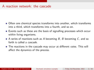
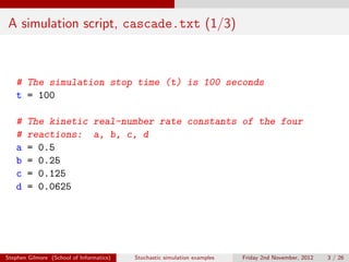
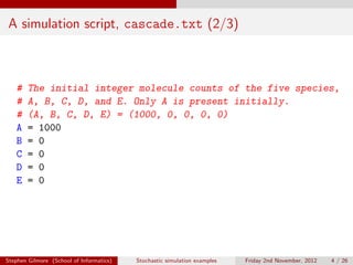
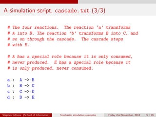
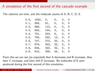
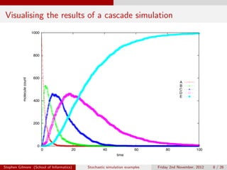
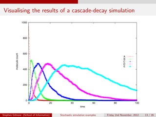
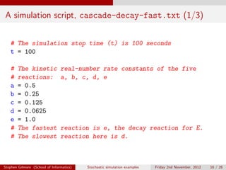
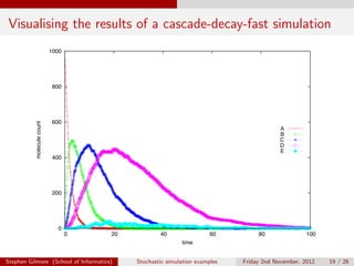
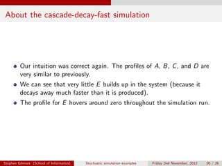
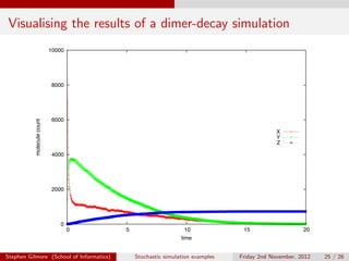
The document describes stochastic simulations of chemical reaction cascades. It discusses simulating a series of reactions (A to B, B to C, etc.) at different rates. A simulation script is provided, and sample output shows species A decreasing while B increases over the first second. The model is expanded to allow species E to decay via a new reaction. Visualizations show this does not affect A-D profiles but changes E's profile. Faster decay of E is also discussed.

1. Computer Science Large Practical:
More Stochastic Simulation Examples
Stephen Gilmore
School of Informatics
Friday 2nd November, 2012
Stephen Gilmore (School of Informatics) Stochastic simulation examples Friday 2nd November, 2012 1 / 26

2. A reaction network: the cascade
Often one chemical species transforms into another, which transforms
into a third, which transforms into a fourth, and so on.
Events such as these are the basis of signalling processes which occur
within living organisms.
A series of reactions such as A becoming B, B becoming C , and so
forth is called a cascade.
The reactions in the cascade may occur at different rates. This will
affect the dynamics of the process.
Stephen Gilmore (School of Informatics) Stochastic simulation examples Friday 2nd November, 2012 2 / 26

3. A simulation script, cascade.txt (1/3)
# The simulation stop time (t) is 100 seconds
t = 100
# The kinetic real-number rate constants of the four
# reactions: a, b, c, d
a = 0.5
b = 0.25
c = 0.125
d = 0.0625
Stephen Gilmore (School of Informatics) Stochastic simulation examples Friday 2nd November, 2012 3 / 26

4. A simulation script, cascade.txt (2/3)
# The initial integer molecule counts of the five species,
# A, B, C, D, and E. Only A is present initially.
# (A, B, C, D, E) = (1000, 0, 0, 0, 0)
A = 1000
B = 0
C = 0
D = 0
E = 0
Stephen Gilmore (School of Informatics) Stochastic simulation examples Friday 2nd November, 2012 4 / 26

5. A simulation script, cascade.txt (3/3)
# The four reactions. The reaction ‘a’ transforms
# A into B. The reaction ’b’ transforms B into C, and
# so on through the cascade. The cascade stops
# with E.
# A has a special role because it is only consumed,
# never produced. E has a special role because it
# is only produced, never consumed.
a : A -> B
b : B -> C
c : C -> D
d : D -> E
Stephen Gilmore (School of Informatics) Stochastic simulation examples Friday 2nd November, 2012 5 / 26

6. A simulation of the first second of the cascade example
The columns are time, and the molecule counts of A, B, C, D, E.
0.0, 1000, 0, 0, 0, 0
0.1, 949, 51, 0, 0, 0
0.2, 888, 112, 0, 0, 0
0.3, 843, 154, 3, 0, 0
0.4, 791, 203, 6, 0, 0
0.5, 756, 232, 12, 0, 0
0.6, 707, 273, 20, 0, 0
0.7, 674, 302, 22, 2, 0
0.8, 644, 322, 32, 2, 0
0.9, 615, 339, 44, 2, 0
From this we can see (as expected) that A decreases and B increases, then
later C increases, and later still D increases. No molecules of E were
produced during the first second of this simulation.
Stephen Gilmore (School of Informatics) Stochastic simulation examples Friday 2nd November, 2012 6 / 26

7. Visualising the results using GNUplot
Store as “cascade.gnu”, plot using “gnuplot cascade.gnu” if results are in “cascade.csv”
set terminal postscript color
set output "cascade.ps"
set key right center
set xlabel "time"
set ylabel "molecule count"
set datafile separator ","
plot
"cascade.csv" using 1:2 with linespoints title "A",
"cascade.csv" using 1:3 with linespoints title "B",
"cascade.csv" using 1:4 with linespoints title "C",
"cascade.csv" using 1:5 with linespoints title "D",
"cascade.csv" using 1:6 with linespoints title "E"
Stephen Gilmore (School of Informatics) Stochastic simulation examples Friday 2nd November, 2012 7 / 26

8. Visualising the results of a cascade simulation
1000
800
600
molecule count
A
B
C
D
E
400
200
0
0 20 40 60 80 100
time
Stephen Gilmore (School of Informatics) Stochastic simulation examples Friday 2nd November, 2012 8 / 26

9. Adding a reaction: allowing E to decay
Now we make a slight change to the model, adding a reaction which
decays E.
We need a new reaction constant for this new reaction. We have
assigned reaction e the slowest rate.
Our intuition should be that this does not make much difference to
the profile of chemical species A, B, C and D in the output, but it
should affect the profile of species E .
Stephen Gilmore (School of Informatics) Stochastic simulation examples Friday 2nd November, 2012 9 / 26

10. A simulation script, cascade-decay.txt (1/3)
# The simulation stop time (t) is 100 seconds
t = 100
# The kinetic real-number rate constants of the five
# reactions: a, b, c, d, e
a = 0.5
b = 0.25
c = 0.125
d = 0.0625
e = 0.03125
Stephen Gilmore (School of Informatics) Stochastic simulation examples Friday 2nd November, 2012 10 / 26

11. A simulation script, cascade-decay.txt (2/3)
This part is exactly the same as cascade.txt
# The initial integer molecule counts of the five species,
# A, B, C, D, and E. Only A is present initially.
# (A, B, C, D, E) = (1000, 0, 0, 0, 0)
A = 1000
B = 0
C = 0
D = 0
E = 0
Stephen Gilmore (School of Informatics) Stochastic simulation examples Friday 2nd November, 2012 11 / 26

12. A simulation script, cascade-decay.txt (3/3)
# The five reactions. The reaction ‘a’ transforms
# A into B. The reaction ’b’ transforms B into C, and
# so on through the cascade. The cascade stops
# with E.
# A has a special role because it is only consumed,
# never produced. E has a special role because it
# decays without producing another output.
a : A -> B
b : B -> C
c : C -> D
d : D -> E
e : E ->
Stephen Gilmore (School of Informatics) Stochastic simulation examples Friday 2nd November, 2012 12 / 26

13. Visualising the results of a cascade-decay simulation
1000
800
600
molecule count
A
B
C
D
E
400
200
0
0 20 40 60 80 100
time
Stephen Gilmore (School of Informatics) Stochastic simulation examples Friday 2nd November, 2012 13 / 26

14. About the cascade-decay simulation
Our intuition was correct. The profiles of A, B, C , and D are very
similar to previously.
Because this is a stochastic simulation which involves pseudo-random
number generation the results will not be exactly the same but they
will be very similar.
We can see that reactions are still occurring right up to the stop-time
of this simulation (t = 100 seconds).
That is perfectly OK in the results. We simulate up to the stop-time
and no further.
Stephen Gilmore (School of Informatics) Stochastic simulation examples Friday 2nd November, 2012 14 / 26

15. Changing a rate in the model
We set the new reaction, e, to be the slowest reaction in the model,
but what if we had chosen it to be the fastest reaction instead?
We can find out how this would affect the results by changing the
rate of reaction e.
Our intuition should be that this again does not make much
difference to the profile of chemical species A, B, C and D in the
output, but it should affect the profile of species E .
Stephen Gilmore (School of Informatics) Stochastic simulation examples Friday 2nd November, 2012 15 / 26

16. A simulation script, cascade-decay-fast.txt (1/3)
# The simulation stop time (t) is 100 seconds
t = 100
# The kinetic real-number rate constants of the five
# reactions: a, b, c, d, e
a = 0.5
b = 0.25
c = 0.125
d = 0.0625
e = 1.0
# The fastest reaction is e, the decay reaction for E.
# The slowest reaction here is d.
Stephen Gilmore (School of Informatics) Stochastic simulation examples Friday 2nd November, 2012 16 / 26

17. A simulation script, cascade-decay-fast.txt (2/3)
This part is exactly the same as cascade-decay.txt
# The initial integer molecule counts of the five species,
# A, B, C, D, and E. Only A is present initially.
# (A, B, C, D, E) = (1000, 0, 0, 0, 0)
A = 1000
B = 0
C = 0
D = 0
E = 0
Stephen Gilmore (School of Informatics) Stochastic simulation examples Friday 2nd November, 2012 17 / 26

18. A simulation script, cascade-decay-fast.txt (3/3)
This part is exactly the same as cascade-decay.txt
# The five reactions. The reaction ‘a’ transforms
# A into B. The reaction ’b’ transforms B into C, and
# so on through the cascade. The cascade stops
# with E.
# A has a special role because it is only consumed,
# never produced. E has a special role because it
# decays without producing another output.
a : A -> B
b : B -> C
c : C -> D
d : D -> E
e : E ->
Stephen Gilmore (School of Informatics) Stochastic simulation examples Friday 2nd November, 2012 18 / 26

19. Visualising the results of a cascade-decay-fast simulation
1000
800
600
molecule count
A
B
C
D
E
400
200
0
0 20 40 60 80 100
time
Stephen Gilmore (School of Informatics) Stochastic simulation examples Friday 2nd November, 2012 19 / 26

20. About the cascade-decay-fast simulation
Our intuition was correct again. The profiles of A, B, C , and D are
very similar to previously.
We can see that very little E builds up in the system (because it
decays away much faster than it is produced).
The profile for E hovers around zero throughout the simulation run.
Stephen Gilmore (School of Informatics) Stochastic simulation examples Friday 2nd November, 2012 20 / 26

21. A dimerisation example
We saw earlier that dimerisation is a special case for the Gillespie
simulation algorithm.
Let’s consider an example which uses dimerisation and also includes a
decay reaction.
Stephen Gilmore (School of Informatics) Stochastic simulation examples Friday 2nd November, 2012 21 / 26

22. A simulation script, dimer-decay.txt (1/3)
# The simulation stop time (t) is 20 seconds
t = 20
# The kinetic real-number rate constants of the four
# reactions: d, x, y, z
d = 1.0
x = 0.002
y = 0.5
z = 0.04
Stephen Gilmore (School of Informatics) Stochastic simulation examples Friday 2nd November, 2012 22 / 26

23. A simulation script, dimer-decay.txt (2/3)
# The initial integer molecule counts of the three
# species, X, Y, and Z. Only X is present initially.
# (X, Y, Z) = (10000, 0, 0)
X = 10000
Y = 0
Z = 0
Stephen Gilmore (School of Informatics) Stochastic simulation examples Friday 2nd November, 2012 23 / 26

24. A simulation script, dimer-decay.txt (3/3)
# The four reactions:
# (d), X can decay to nothing;
# (x), two molecules of X can bind to form Y;
# (y), Y can unbind to give two molecules of X; and
# (z), a molecule of Y can produce a molecule of Z.
d : X ->
x : X + X -> Y
y : Y -> X + X
z : Y -> Z
Stephen Gilmore (School of Informatics) Stochastic simulation examples Friday 2nd November, 2012 24 / 26

25. Visualising the results of a dimer-decay simulation
10000
8000
6000
molecule count
X
Y
Z
4000
2000
0
0 5 10 15 20
time
Stephen Gilmore (School of Informatics) Stochastic simulation examples Friday 2nd November, 2012 25 / 26

26. Summary
We have seen some examples of simulation scripts involving cascades
and dimerisation.
Try creating some of your own. For example:
A cascade which involves more species.
A cascade where every species can decay, not just the last one.
A dimerisation example without a decay reaction.
Stephen Gilmore (School of Informatics) Stochastic simulation examples Friday 2nd November, 2012 26 / 26