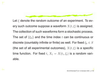
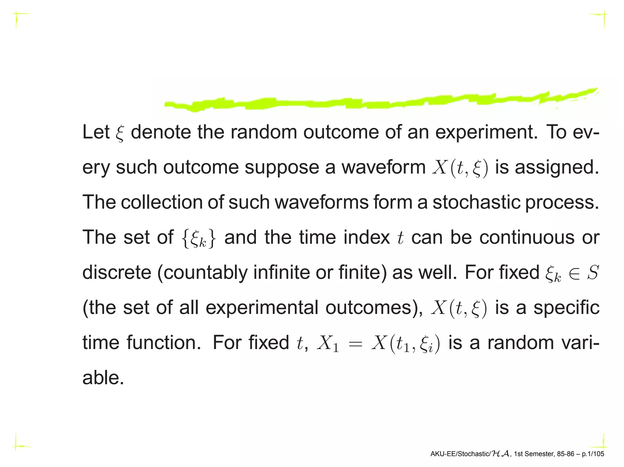
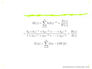
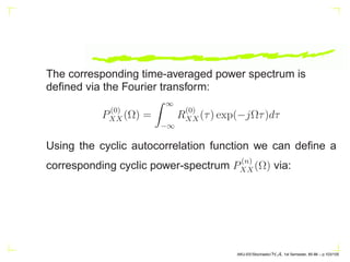
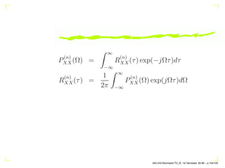
The document discusses stochastic processes, defining outcomes of experiments as waveforms that create random variables dependent on time. It covers key concepts such as mean functions, correlation functions, and the specifications required to analyze these processes. The distinction between strict-sense stationary and wide-sense stationary processes, along with the properties of Gaussian processes, is also elaborated.

![1. RXX(t1, t2) = R∗
XX(t2, t1) = [E{X(t2)X∗
(t1)}]∗
2. RXX(t, t) = E{|X(t)|2
} > 0.
3.
n
P
i=1
n
P
j=1
aia∗
j RXX(ti, tj) ≥ 0.
CXX(t1, t2) = RXX(t1, t2) − µX(t1)µ∗
X(t2)
AKU-EE/Stochastic/HA, 1st Semester, 85-86 – p.7/105](https://image.slidesharecdn.com/stoch1-210301121813/85/Stochastic-Processes-part-1-7-320.jpg)
![Example:
z =
Z T
−T
X(t)dt
E[|z|2
] =
Z T
−T
Z T
−T
E{X(t1)X∗
(t2)}dt1dt2
=
Z T
−T
Z T
−T
RXX(t1, t2)dt1dt2
AKU-EE/Stochastic/HA, 1st Semester, 85-86 – p.8/105](https://image.slidesharecdn.com/stoch1-210301121813/85/Stochastic-Processes-part-1-8-320.jpg)
![For a first-order strict sense stationary process,
fX(x, t) ≡ fX(x, t + c)
for c = −t,
fX(x, t) = fX(x) (2)
the first-order density of X(t) is independent of t. In that
case
E[X(t)] =
Z +∞
−∞
xf(x)dx = µ, a constant.
AKU-EE/Stochastic/HA, 1st Semester, 85-86 – p.13/105](https://image.slidesharecdn.com/stoch1-210301121813/85/Stochastic-Processes-part-1-13-320.jpg)

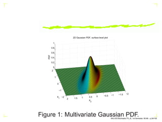
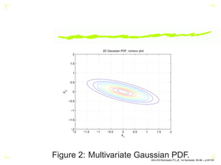
![N-dim Gaussian
C=[.5,-.15;-.15,.2]; mu=[1 -1];
[X1,X2] = meshgrid(linspace(-2,2,100)’,
linspace(-2,2,100)’);
X = [X1(:) X2(:)];
p = mvnpdf(X, mu, C);
surf(X1,X2,reshape(p,100,100));
contour(X1,X2,reshape(p,100,100));
AKU-EE/Stochastic/HA, 1st Semester, 85-86 – p.23/105](https://image.slidesharecdn.com/stoch1-210301121813/85/Stochastic-Processes-part-1-23-320.jpg)
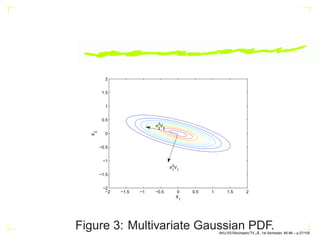
![C = V DV H
, V = [V1 V2]
C =
0.5 −.15
−0.15 0.2
V =
0.31625 −.9487
−0.9487 0.3162
D =
0.05 0
0 0.55
AKU-EE/Stochastic/HA, 1st Semester, 85-86 – p.26/105](https://image.slidesharecdn.com/stoch1-210301121813/85/Stochastic-Processes-part-1-26-320.jpg)

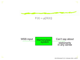
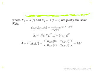
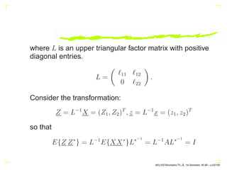
![If X(t) is a zero mean stationary Gaussian process, and
Y (t) = g{X(t)}, where g(·) represents a nonlinear
memoryless device, then
RXY (τ) = ηRXX(τ), η = E{g′
(X)}.
Proof:
RXY (τ) = E{X(t)Y (t − τ)} = E[X(t)g{X(t − τ)}]
=
Z Z
x1g(x2)fX1X2 (x1, x2)dx1dx2, (5)
AKU-EE/Stochastic/HA, 1st Semester, 85-86 – p.40/105](https://image.slidesharecdn.com/stoch1-210301121813/85/Stochastic-Processes-part-1-40-320.jpg)


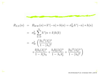
![E[N(t)] = µW
Z +∞
−∞
h(τ)dτ = a constant
RNN (τ) = qδ(τ) ∗ h∗
(−τ) ∗ h(τ)
= qh∗
(−τ) ∗ h(τ) = qρ(τ)
ρ(τ) = h(τ) ∗ h∗
(−τ) =
Z +∞
−∞
h(α)h∗
(α + τ)dα.
AKU-EE/Stochastic/HA, 1st Semester, 85-86 – p.54/105](https://image.slidesharecdn.com/stoch1-210301121813/85/Stochastic-Processes-part-1-54-320.jpg)
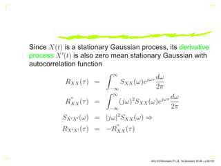
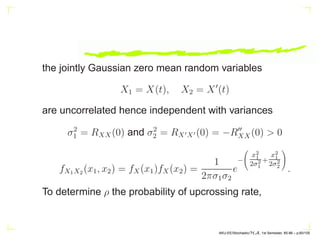
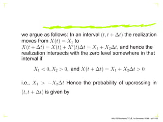
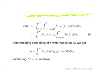
![Further X(t) and X′
(t) and are jointly Gaussian stationary
processes, and since
RXX′ (τ) = −
dRXX(τ)
dτ
,
RXX′ (−τ) = −
dRXX(−τ)
d(−τ)
=
dRXX(τ)
dτ
= −RXX′ (τ)
which for τ = 0 gives
RXX′ (0) = 0 ⇒ E[X(t)X′
(t)] = 0
AKU-EE/Stochastic/HA, 1st Semester, 85-86 – p.59/105](https://image.slidesharecdn.com/stoch1-210301121813/85/Stochastic-Processes-part-1-59-320.jpg)
![WSS:
E{X(nT)} = µ, a constant
E[X{(k + n)T}X∗
{(k)T}] = R(n) = rn = r∗
−n
AKU-EE/Stochastic/HA, 1st Semester, 85-86 – p.66/105](https://image.slidesharecdn.com/stoch1-210301121813/85/Stochastic-Processes-part-1-66-320.jpg)
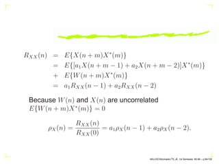


![RXX(n) = E{X(n + m)X∗
(m)}
= E{[a1X(n + m − 1) + a2X(n + m − 2)]X∗
(m)}
+ E{W(n + m)X∗
(m)}
= a1RXX(n − 1) + a2RXX(n − 2)
Because W(n) and X(n) are uncorrelated
E{W(n + m)X∗
(m)} = 0
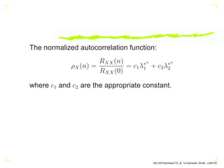
ρX(n) =
RXX(n)
RXX(0)
= a1ρX(n − 1) + a2ρX(n − 2).
AKU-EE/Stochastic/HA, 1st Semester, 85-86 – p.84/105](https://image.slidesharecdn.com/stoch1-210301121813/85/Stochastic-Processes-part-1-94-320.jpg)


![Digital Signal Processing[ECEG-3171]-Ch1_L03](https://cdn.slidesharecdn.com/ss_thumbnails/dspl3-180427094423-thumbnail.jpg?width=640&height=640&fit=bounds)