Download as PDF, PPTX
![ned
expectation E[X]
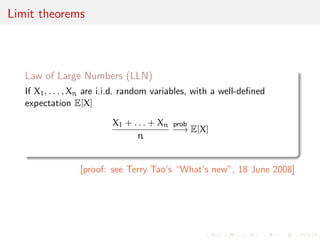
X1 + . . . + Xn
n
prob
! E[X]
[proof: see Terry Tao's What's new, 18 June 2008]](https://image.slidesharecdn.com/models-140923111143-phpapp02/85/Statistics-1-estimation-Chapter-1-Models-7-320.jpg)
![ned
expectation E[X]
X1 + . . . + Xn
n
a.s.
! E[X]
[proof: see Terry Tao's What's new, 18 June 2008]](https://image.slidesharecdn.com/models-140923111143-phpapp02/85/Statistics-1-estimation-Chapter-1-Models-9-320.jpg)
![ned
expectation E[X]
X1 + . . . + Xn
n
a.s.
! E[X]
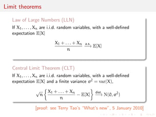
Central Limit Theorem (CLT)
If X1, . . . ,Xn are i.i.d. random variables, with a well-de](https://image.slidesharecdn.com/models-140923111143-phpapp02/85/Statistics-1-estimation-Chapter-1-Models-11-320.jpg)
![ned
expectation E[X] and a](https://image.slidesharecdn.com/models-140923111143-phpapp02/85/Statistics-1-estimation-Chapter-1-Models-12-320.jpg)
![X1 + . . . + Xn
n
- E[X]
dist.
! N(0, 2)
[proof: see Terry Tao's What's new, 5 January 2010]](https://image.slidesharecdn.com/models-140923111143-phpapp02/85/Statistics-1-estimation-Chapter-1-Models-14-320.jpg)
![ned
expectation E[X] and a](https://image.slidesharecdn.com/models-140923111143-phpapp02/85/Statistics-1-estimation-Chapter-1-Models-16-320.jpg)
![X1 + . . . + Xn
n
- E[X]
dist.
! N(0, 2)
[proof: see Terry Tao's What's new, 5 January 2010]
Continuity Theorem
If
Xn
dist.
! a
and g is continuous at a, then
g(Xn)
dist.
! g(a)](https://image.slidesharecdn.com/models-140923111143-phpapp02/85/Statistics-1-estimation-Chapter-1-Models-18-320.jpg)
![ned
expectation E[X] and a](https://image.slidesharecdn.com/models-140923111143-phpapp02/85/Statistics-1-estimation-Chapter-1-Models-20-320.jpg)
![X1 + . . . + Xn
n
- E[X]
dist.
! N(0, 2)
[proof: see Terry Tao's What's new, 5 January 2010]
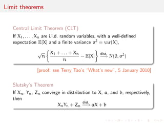
Slutsky's Theorem
If Xn, Yn, Zn converge in distribution to X, a, and b, respectively,
then
XnYn + Zn
dist.
! aX + b](https://image.slidesharecdn.com/models-140923111143-phpapp02/85/Statistics-1-estimation-Chapter-1-Models-22-320.jpg)
![ned
expectation E[X] and a](https://image.slidesharecdn.com/models-140923111143-phpapp02/85/Statistics-1-estimation-Chapter-1-Models-24-320.jpg)
![X1 + . . . + Xn
n
- E[X]
dist.
! N(0, 2)
[proof: see Terry Tao's What's new, 5 January 2010]
Delta method's Theorem
If p
nfXn - g
dist.
! Np(0,
)
and g : Rp ! Rq is a continuously dierentiable function on a
neighbourhood of 2 Rp, with a non-zero gradient rg(), then
p
n fg(Xn) - g()g
dist.
! Nq(0,rg()T
rg())](https://image.slidesharecdn.com/models-140923111143-phpapp02/85/Statistics-1-estimation-Chapter-1-Models-26-320.jpg)
![Non-parametric models
In non-parametric models, there may still be constraints on the
range of F`s as for instance
EF[YjX = x] = (](https://image.slidesharecdn.com/models-140923111143-phpapp02/85/Statistics-1-estimation-Chapter-1-Models-35-320.jpg)
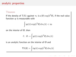
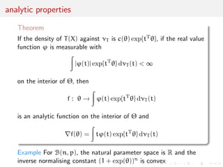
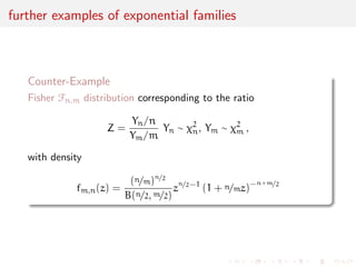
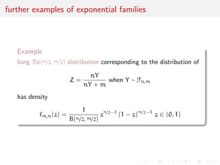
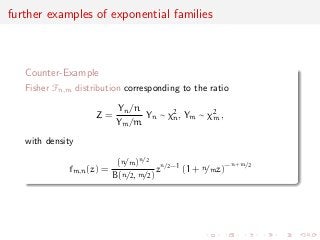
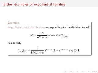

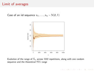
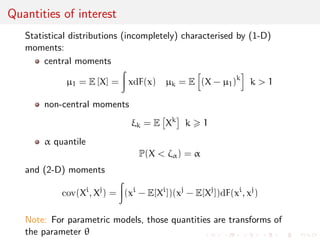
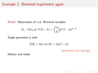
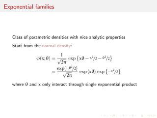
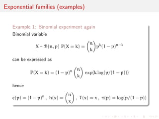
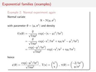
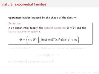
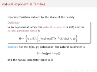
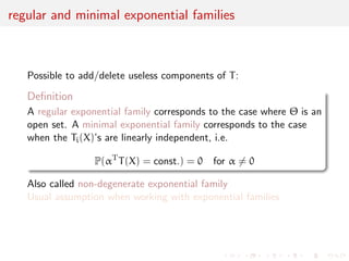
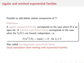
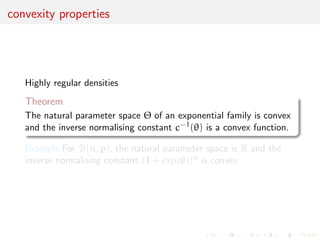
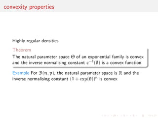
The document discusses statistical models and exponential families. It states that for most of the course, data is assumed to be a random sample from a distribution F. Repetition of observations via the law of large numbers and central limit theorem increases information about F. Exponential families are a class of parametric distributions with convenient analytic properties, where the density can be written as a function of natural parameters in an exponential form. Examples of exponential families include the binomial and normal distributions.