Download as PDF, PPTX


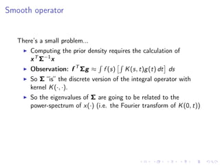
![“except as a source of approximations [...] asymptotics have
no practical utility at best and are misleading at worst”
So to make the asymptotics work as we get more data, we
need to specify the GP smoothness correctly
Awkward!
A work around: Choose a very smooth GP e.g.
k(s, t) = exp(−κ(s − t)2
)
and put a good prior on κ. (van der Vaart & van Zanten,
2009)
Bayes to the rescue!](https://image.slidesharecdn.com/bigmodel-151215214112/85/Big-model-big-data-20-320.jpg)
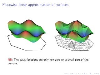

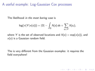

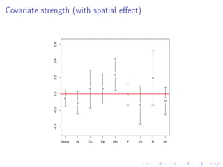

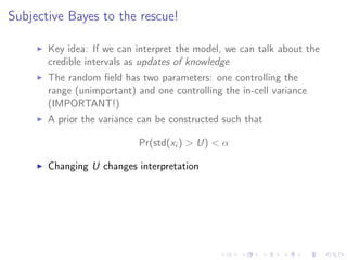


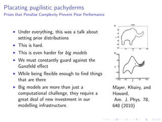

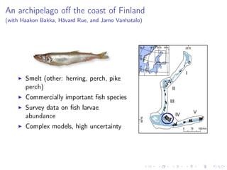
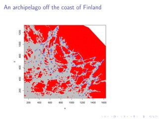
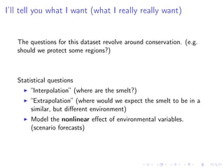
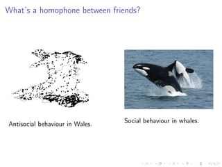
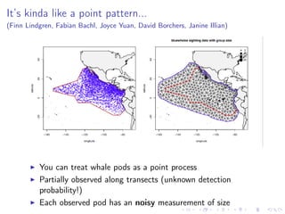
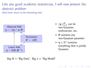
The document discusses the complexities and challenges of modeling large datasets, particularly in ecological contexts, emphasizing the necessity of investment in both modeling and computational strategies to address uncertainties. It illustrates specific examples involving fish population surveys and whale pod observations to demonstrate statistical questions related to detection probabilities and inference in the presence of noise and incomplete data. Furthermore, the text highlights the limitations and nuances of Gaussian processes in modeling non-linear effects, advocating for Bayesian approaches to enhance interpretability and manage uncertainty in ecological modeling.


![Inference in generative models using the Wasserstein distance [[INI]](https://cdn.slidesharecdn.com/ss_thumbnails/inewton-170706120746-thumbnail.jpg?width=640&height=640&fit=bounds)


![Polymer [ बहुलक ] Chemistry Notes PDF - Irfanullah Mehar - JJ Sir Chemistry.pdf](https://cdn.slidesharecdn.com/ss_thumbnails/polymerchemistrynotespdf-irfanullahmehar-jjsirchemistry-260210172118-3f9b37f7-thumbnail.jpg?width=640&height=640&fit=bounds)


