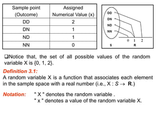
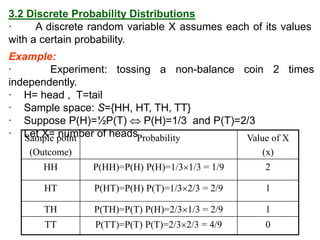
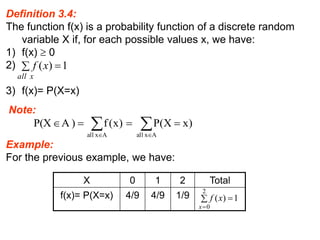
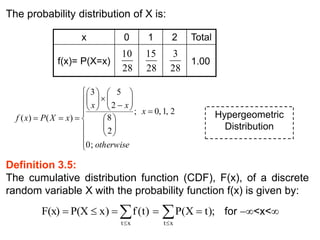
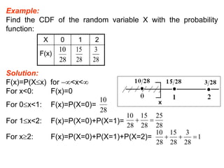
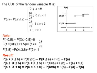
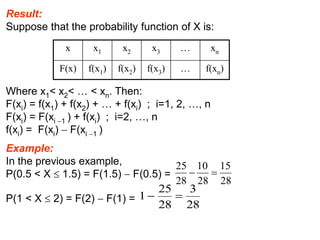
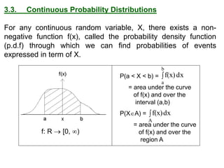
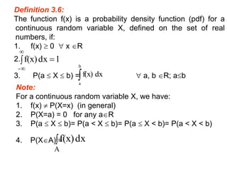
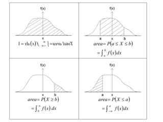
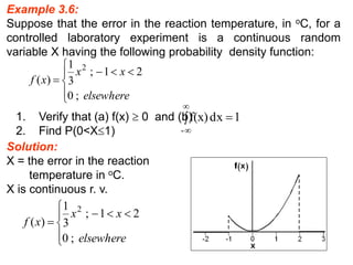
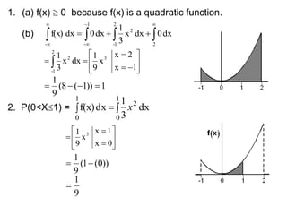
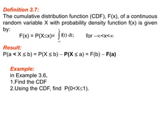
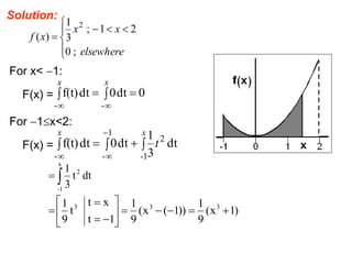
The document summarizes key concepts about random variables and probability distributions. It defines a random variable as a function that assigns numerical values to outcomes of a statistical experiment. Random variables can be discrete, taking on countable values, or continuous, having values on a continuous scale. For discrete random variables, the probabilities of each value are specified by the probability mass function (PMF). For continuous random variables, the probability density function (PDF) gives the probability of values in an interval as the area under the curve of the function. The cumulative distribution function (CDF) gives the probability that a random variable is less than or equal to a value. 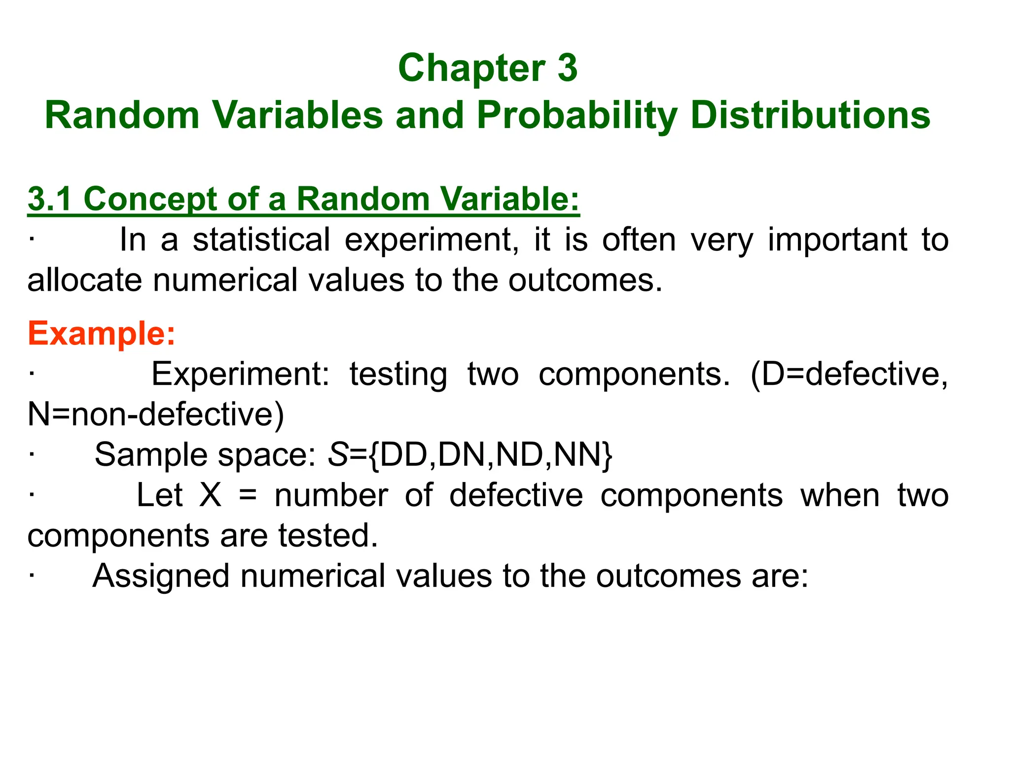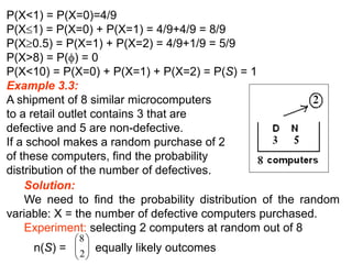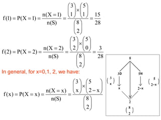An example calculates the PMF of the number of defective computers selected in

1. Chapter 3
Random Variables and Probability Distributions
3.1 Concept of a Random Variable:
· In a statistical experiment, it is often very important to
allocate numerical values to the outcomes.
Example:
· Experiment: testing two components. (D=defective,
N=non-defective)
· Sample space: S={DD,DN,ND,NN}
· Let X = number of defective components when two
components are tested.
· Assigned numerical values to the outcomes are:

2. Sample point
(Outcome)
Assigned
Numerical Value (x)
DD 2
DN 1
ND 1
NN 0
Notice that, the set of all possible values of the random
variable X is {0, 1, 2}.
Definition 3.1:
A random variable X is a function that associates each element
in the sample space with a real number (i.e., X : S  R.)
Notation: " X " denotes the random variable .
" x " denotes a value of the random variable X.

3. Types of Random Variables:
· A random variable X is called a discrete random
variable if its set of possible values is countable, i.e.,
.x  {x1, x2, …, xn} or x  {x1, x2, …}
· A random variable X is called a continuous random
variable if it can take values on a continuous scale, i.e.,
.x  {x: a < x < b; a, b R}
· In most practical problems:
o A discrete random variable represents count data, such
as the number of defectives in a sample of k items.
o A continuous random variable represents measured
data, such as height.

4. 3.2 Discrete Probability Distributions
· A discrete random variable X assumes each of its values
with a certain probability.
Example:
· Experiment: tossing a non-balance coin 2 times
independently.
· H= head , T=tail
· Sample space: S={HH, HT, TH, TT}
· Suppose P(H)=½P(T)  P(H)=1/3 and P(T)=2/3
· Let X= number of heads
Sample point
(Outcome)
Probability Value of X
(x)
HH P(HH)=P(H) P(H)=1/31/3 = 1/9 2
HT P(HT)=P(H) P(T)=1/32/3 = 2/9 1
TH P(TH)=P(T) P(H)=2/31/3 = 2/9 1
TT P(TT)=P(T) P(T)=2/32/3 = 4/9 0

5. · The possible values of X are: 0, 1, and 2.
· X is a discrete random variable.
· Define the following events:
Event (X=x) Probability = P(X=x)
(X=0)={TT} P(X=0) = P(TT)=4/9
(X=1)={HT,TH} P(X=1) =P(HT)+P(TH)=2/9+2/9=4/9
(X=2)={HH} P(X=2) = P(HH)= 1/9
· The possible values of X with their probabilities are:
X 0 1 2 Total
P(X=x)=f(x) 4/9 4/9 1/9 1.00
The function f(x)=P(X=x) is called the probability function
(probability distribution) of the discrete random variable X.

6. Definition 3.4:
The function f(x) is a probability function of a discrete random
variable X if, for each possible values x, we have:
1) f(x)  0
2)
3) f(x)= P(X=x)
1
)
( 

x
all
x
f
Note:

 





A
x
all
A
x
all
)
x
X
(
P
)
x
(
f
)
A
P(X
Example:
For the previous example, we have:
1/9
4/9
4/9
f(x)= P(X=x)
Total
2
1
0
X
1
)
(
2
0



x
x
f

7. P(X<1) = P(X=0)=4/9
P(X1) = P(X=0) + P(X=1) = 4/9+4/9 = 8/9
P(X0.5) = P(X=1) + P(X=2) = 4/9+1/9 = 5/9
P(X>8) = P() = 0
P(X<10) = P(X=0) + P(X=1) + P(X=2) = P(S) = 1
Example 3.3:
A shipment of 8 similar microcomputers
to a retail outlet contains 3 that are
defective and 5 are non-defective.
If a school makes a random purchase of 2
of these computers, find the probability
distribution of the number of defectives.
Solution:
We need to find the probability distribution of the random
variable: X = the number of defective computers purchased.
Experiment: selecting 2 computers at random out of 8
n(S) = equally likely outcomes








2
8

8. The possible values of X are: x=0, 1, 2.
Consider the events:






















2
5
0
3
0)
n(X
2N}
and
{0D
0)
(X






















1
5
1
3
1)
n(X
1N}
and
{1D
1)
(X






















0
5
2
3
2)
n(X
0N}
and
{2D
2)
(X
28
10
2
8
2
5
0
3
)
S
(
n
)
0
X
(
n
)
0
X
(
P
)
0
(
f 































9. 28
15
2
8
1
5
1
3
)
S
(
n
)
1
X
(
n
)
1
X
(
P
)
1
(
f 






























28
3
2
8
0
5
2
3
)
S
(
n
)
2
X
(
n
)
2
X
(
P
)
2
(
f 






























In general, for x=0,1, 2, we have:































2
8
x
2
5
x
3
)
S
(
n
)
x
X
(
n
)
x
X
(
P
)
x
(
f

10. The probability distribution of X is:
x 0 1 2 Total
f(x)= P(X=x)
28
10
28
15
28
3







































otherwise
x
x
x
x
X
P
x
f
;
0
2
,
1
,
0
;
2
8
2
5
3
)
(
)
( Hypergeometric
Distribution
Definition 3.5:
The cumulative distribution function (CDF), F(x), of a discrete
random variable X with the probability function f(x) is given by:
;
)
t
X
(
P
)
t
(
f
)
x
P(X
F(x)
x
t
x
t

 






 for <x<
1.00

11. Example:
Find the CDF of the random variable X with the probability
function:
X 0 1 2
F(x)
28
10
28
15
28
3
Solution:
F(x)=P(Xx) for <x<
For x<0: F(x)=0
For 0x<1: F(x)=P(X=0)=
28
10
28
25
28
15
28
10


For 1x<2: F(x)=P(X=0)+P(X=1)=
For x2: F(x)=P(X=0)+P(X=1)+P(X=2)= 1
28
3
28
15
28
10




12. The CDF of the random variable X is:


















2
;
1
2
1
;
28
25
1
0
;
28
10
0
;
0
)
(
)
(
x
x
x
x
x
X
P
x
F
Note:
F(0.5) = P(X0.5)=0
F(1.5)=P(X1.5)=F(1) =
F(3.8) =P(X3.8)=F(2)= 1
28
25
Result:
P(a < X  b) = P(X  b)  P(X  a) = F(b)  F(a)
P(a  X  b) = P(a < X  b) + P(X=a) = F(b)  F(a) + f(a)
P(a < X < b) = P(a < X  b)  P(X=b) = F(b)  F(a)  f(b)

13. Result:
Suppose that the probability function of X is:
x x1 x2 x3 … xn
F(x) f(x1) f(x2) f(x3) … f(xn)
Where x1< x2< … < xn. Then:
F(xi) = f(x1) + f(x2) + … + f(xi) ; i=1, 2, …, n
F(xi) = F(xi 1 ) + f(xi) ; i=2, …, n
f(xi) = F(xi)  F(xi 1 )
Example:
In the previous example,
P(0.5 < X  1.5) = F(1.5)  F(0.5) =
P(1 < X  2) = F(2)  F(1) =
28
15
28
10
28
25


28
3
28
25
1 


14. 3.3. Continuous Probability Distributions
For any continuous random variable, X, there exists a non-
negative function f(x), called the probability density function
(p.d.f) through which we can find probabilities of events
expressed in term of X.
f: R  [0, )
P(a < X < b) =
= area under the curve
of f(x) and over the
interval (a,b)
P(XA) =
= area under the curve
of f(x) and over the
region A

b
a
dx
f(x)

A
dx
f(x)

15. Definition 3.6:
The function f(x) is a probability density function (pdf) for a
continuous random variable X, defined on the set of real
numbers, if:
1. f(x)  0  x R
2.
3. P(a  X  b) =  a, b R; ab
1
dx
f(x)
-





b
a
dx
f(x)
Note:
For a continuous random variable X, we have:
1. f(x)  P(X=x) (in general)
2. P(X=a) = 0 for any aR
3. P(a  X  b)= P(a < X  b)= P(a  X < b)= P(a < X < b)
4. P(XA) =

A
dx
f(x)

16. 

1  


d
x x f a
r
e
a T
o
t
a
l  
 





b
a
dx
x
f
b
X
a
P
area
 
 





b
dx
x
f
b
X
P
area  
 
 




a
dx
x
f
a
X
P
area

17. Example 3.6:
Suppose that the error in the reaction temperature, in oC, for a
controlled laboratory experiment is a continuous random
variable X having the following probability density function:









elsewhere
x
x
x
f
;
0
2
1
;
3
1
)
(
2
1. Verify that (a) f(x)  0 and (b)
2. Find P(0<X1)
1
dx
f(x)
-




Solution:
X = the error in the reaction
temperature in oC.
X is continuous r. v.









elsewhere
x
x
x
f
;
0
2
1
;
3
1
)
(
2

18. 1. (a) f(x)  0 because f(x) is a quadratic function.
(b) 











2
2
1
-
2
1
-
-
dx
0
dx
x
3
1
dx
0
dx
f(x)










  1
x
2
x
x
9
1
dx
x
3
1 3
2
1
-
2
1
))
1
(
8
(
9
1




2. P(0<X1) = 


1
0
2
1
0
dx
3
1
dx
f(x) x









0
x
1
x
x
9
1 3
))
0
(
1
(
9
1


9
1


19. Definition 3.7:
The cumulative distribution function (CDF), F(x), of a continuous
random variable X with probability density function f(x) is given
by:
F(x) = P(Xx)= for <x<
;
dt
f(t)
x
-


Result:
P(a < X  b) = P(X  b)  P(X  a) = F(b)  F(a)
Example:
in Example 3.6,
1.Find the CDF
2.Using the CDF, find P(0<X1).

20. Solution:









elsewhere
x
x
x
f
;
0
2
1
;
3
1
)
(
2
For x< 1:
F(x) = 0
dt
0
dt
f(t)
-
-






x
x
For 1x<2:
F(x) = 







x
x
t
1
-
2
1
-
-
dt
3
1
dt
0
dt
f(t)


x
1
-
2
dt
t
3
1
)
1
x
(
9
1
))
1
(
x
(
9
1
1
t
x
t
t
9
1 3
3
3
















21. For x2:
F(x) = =
dt
0
dt
t
3
1
dt
0
dt
f(t)
x
2
2
1
-
2
1
-
x
-



 





1
dt
t
3
1
2
1
-
2


Therefore, the CDF is:

















2
;
1
2
1
;
)
1
(
9
1
1
;
0
)
(
)
( 3
x
x
x
x
x
X
P
x
F
2. Using the CDF,
P(0<X1) = F(1)  F(0) =
9
1
9
1
9
2

