Download as PDF, PPTX
![Chapter 3 :
Likelihood function and inference
[0]
4 Likelihood function and inference
The likelihood
Information and curvature
Suciency and ancilarity
Maximum likelihood estimation
Non-regular models
EM algorithm](https://image.slidesharecdn.com/like-141026114245-conversion-gate02/85/Statistics-1-estimation-Chapter-3-likelihood-function-and-likelihood-estimation-1-320.jpg)
![Chapter 3 :
Likelihood function and inference
[0]
4 Likelihood function and inference
The likelihood
Information and curvature
Suciency and ancilarity
Maximum likelihood estimation
Non-regular models
EM algorithm](https://image.slidesharecdn.com/like-141026114245-conversion-gate02/75/Statistics-1-estimation-Chapter-3-likelihood-function-and-likelihood-estimation-1-2048.jpg)
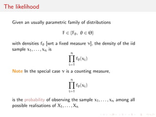
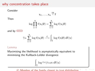
![xed measure ], the density of the iid
sample x1, . . . , xn is
Yn
i=1
f(xi)
Note In the special case is a counting measure,
Yn
i=1
f(xi)
is the probability of observing the sample x1, . . . , xn among all
possible realisations of X1, . . . ,Xn](https://image.slidesharecdn.com/like-141026114245-conversion-gate02/85/Statistics-1-estimation-Chapter-3-likelihood-function-and-likelihood-estimation-3-320.jpg)
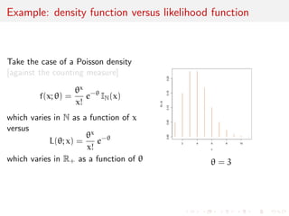
![Example: density function versus likelihood function
Take the case of a Poisson density
[against the counting measure]
f(x; ) =
x
x!
e- IN(x)
which varies in N as a function of x
versus
L(; x) =
x
x!
e-
which varies in R+ as a function of = 3](https://image.slidesharecdn.com/like-141026114245-conversion-gate02/85/Statistics-1-estimation-Chapter-3-likelihood-function-and-likelihood-estimation-6-320.jpg)
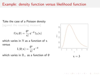
![Example: density function versus likelihood function
Take the case of a Poisson density
[against the counting measure]
f(x; ) =
x
x!
e- IN(x)
which varies in N as a function of x
versus
L(; x) =
x
x!
e-
which varies in R+ as a function of x = 3](https://image.slidesharecdn.com/like-141026114245-conversion-gate02/85/Statistics-1-estimation-Chapter-3-likelihood-function-and-likelihood-estimation-7-320.jpg)
![Example: density function versus likelihood function
Take the case of a Normal N(0, )
density [against the Lebesgue measure]
f(x; ) =
1
p
2
e-x2=2 IR(x)
which varies in R as a function of x
versus
L(; x) =
1
p
2
e-x2=2
which varies in R+ as a function of
= 2](https://image.slidesharecdn.com/like-141026114245-conversion-gate02/85/Statistics-1-estimation-Chapter-3-likelihood-function-and-likelihood-estimation-8-320.jpg)
![Example: density function versus likelihood function
Take the case of a Normal N(0, )
density [against the Lebesgue measure]
f(x; ) =
1
p
2
e-x2=2 IR(x)
which varies in R as a function of x
versus
L(; x) =
1
p
2
e-x2=2
which varies in R+ as a function of
x = 2](https://image.slidesharecdn.com/like-141026114245-conversion-gate02/85/Statistics-1-estimation-Chapter-3-likelihood-function-and-likelihood-estimation-9-320.jpg)
![Example: density function versus likelihood function
Take the case of a Normal N(0, 1=)
density [against the Lebesgue measure]
f(x; ) =
p
p
2
e-x2=2 IR(x)
which varies in R as a function of x
versus
L(; x) =
p
p
2
e-x2=2 IR(x)
which varies in R+ as a function of
= 1=2](https://image.slidesharecdn.com/like-141026114245-conversion-gate02/85/Statistics-1-estimation-Chapter-3-likelihood-function-and-likelihood-estimation-10-320.jpg)
![Example: density function versus likelihood function
Take the case of a Normal N(0, 1=)
density [against the Lebesgue measure]
f(x; ) =
p
p
2
e-x2=2 IR(x)
which varies in R as a function of x
versus
L(; x) =
p
p
2
e-x2=2 IR(x)
which varies in R+ as a function of
x = 1=2](https://image.slidesharecdn.com/like-141026114245-conversion-gate02/85/Statistics-1-estimation-Chapter-3-likelihood-function-and-likelihood-estimation-11-320.jpg)
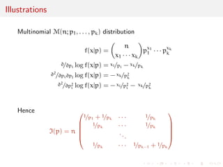
![Example: Hardy-Weinberg equilibrium
Population genetics:
Genotypes of biallelic genes AA, Aa, and aa
sample frequencies nAA, nAa and naa
multinomial model M(n; pAA, pAa, paa)
related to population proportion of A alleles, pA:
pAA = p2
A , pAa = 2pA(1 - pA) , paa = (1 - pA)2
likelihood
L(pAjnAA, nAa, naa) / p2nAA
A [2pA(1 - pA)]nAa(1 - pA)2naa
[Boos Stefanski, 2013]](https://image.slidesharecdn.com/like-141026114245-conversion-gate02/85/Statistics-1-estimation-Chapter-3-likelihood-function-and-likelihood-estimation-12-320.jpg)
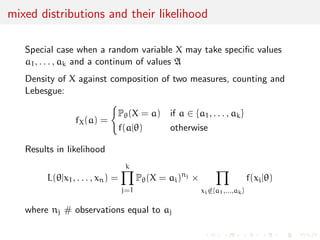
![c values
a1, . . . , ak and a continum of values A
Example: Rainfall at a given spot on a given day may be zero with
positive probability p0 [it did not rain!] or an arbitrary number
between 0 and 100 [capacity of measurement container] or 100
with positive probability p100 [container full]](https://image.slidesharecdn.com/like-141026114245-conversion-gate02/85/Statistics-1-estimation-Chapter-3-likelihood-function-and-likelihood-estimation-14-320.jpg)

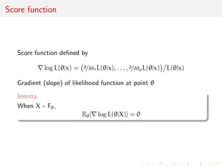
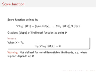
![ned by
rlog L(jx) =
@=@1L(jx), . . . , @=@pL(jx)
L(jx)
Gradient (slope) of likelihood function at point
lemma
When X F,
E[rlog L(jX)] = 0](https://image.slidesharecdn.com/like-141026114245-conversion-gate02/85/Statistics-1-estimation-Chapter-3-likelihood-function-and-likelihood-estimation-28-320.jpg)
![ned by
rlog L(jx) =
@=@1L(jx), . . . , @=@pL(jx)
L(jx)
Gradient (slope) of likelihood function at point
lemma
When X F,
E[rlog L(jX)] = 0](https://image.slidesharecdn.com/like-141026114245-conversion-gate02/85/Statistics-1-estimation-Chapter-3-likelihood-function-and-likelihood-estimation-30-320.jpg)
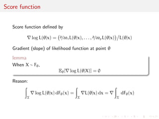
![ned by
rlog L(jx) =
@=@1L(jx), . . . , @=@pL(jx)
L(jx)
Gradient (slope) of likelihood function at point
lemma
When X F,
E[rlog L(jX)] = 0
Reason:
Z
X
rlog L(jx) dF(x) =
Z
X
rL(jx) dx = r
Z
X
dF(x)](https://image.slidesharecdn.com/like-141026114245-conversion-gate02/85/Statistics-1-estimation-Chapter-3-likelihood-function-and-likelihood-estimation-32-320.jpg)
![ned by
rlog L(jx) =
@=@1L(jx), . . . , @=@pL(jx)
L(jx)
Gradient (slope) of likelihood function at point
lemma
When X F,
E[rlog L(jX)] = 0
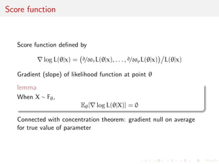
Connected with concentration theorem: gradient null on average
for true value of parameter](https://image.slidesharecdn.com/like-141026114245-conversion-gate02/85/Statistics-1-estimation-Chapter-3-likelihood-function-and-likelihood-estimation-34-320.jpg)
![ned by
rlog L(jx) =
@=@1L(jx), . . . , @=@pL(jx)
L(jx)
Gradient (slope) of likelihood function at point
lemma
When X F,
E[rlog L(jX)] = 0
Warning: Not de](https://image.slidesharecdn.com/like-141026114245-conversion-gate02/85/Statistics-1-estimation-Chapter-3-likelihood-function-and-likelihood-estimation-36-320.jpg)
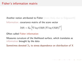
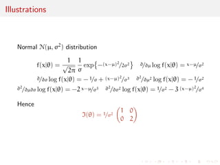
![Fisher's information matrix
Another notion attributed to Fisher [more likely due to Edgeworth]
Information: covariance matrix of the score vector
I() = E
h
rlog f(Xj) frlog f(Xj)gT
i
Often called Fisher information
Measures curvature of the likelihood surface, which translates as
information brought by the data
Sometimes denoted IX to stress dependence on distribution of X](https://image.slidesharecdn.com/like-141026114245-conversion-gate02/85/Statistics-1-estimation-Chapter-3-likelihood-function-and-likelihood-estimation-38-320.jpg)
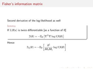
![Fisher's information matrix
Second derivative of the log-likelihood as well
lemma
If L(jx) is twice dierentiable [as a function of ]
I() = -E
rTrlog f(Xj)
Hence
Iij() = -E
@2
@i@j
log f(Xj)](https://image.slidesharecdn.com/like-141026114245-conversion-gate02/85/Statistics-1-estimation-Chapter-3-likelihood-function-and-likelihood-estimation-39-320.jpg)
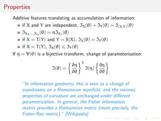
![@
@
In information geometry, this is seen as a change of
coordinates on a Riemannian manifold, and the intrinsic
properties of curvature are unchanged under dierent
parametrization. In general, the Fisher information
matrix provides a Riemannian metric (more precisely, the
Fisher-Rao metric). [Wikipedia]](https://image.slidesharecdn.com/like-141026114245-conversion-gate02/85/Statistics-1-estimation-Chapter-3-likelihood-function-and-likelihood-estimation-46-320.jpg)
![@
@
In information geometry, this is seen as a change of
coordinates on a Riemannian manifold, and the intrinsic
properties of curvature are unchanged under dierent
parametrization. In general, the Fisher information
matrix provides a Riemannian metric (more precisely, the
Fisher-Rao metric). [Wikipedia]](https://image.slidesharecdn.com/like-141026114245-conversion-gate02/85/Statistics-1-estimation-Chapter-3-likelihood-function-and-likelihood-estimation-49-320.jpg)
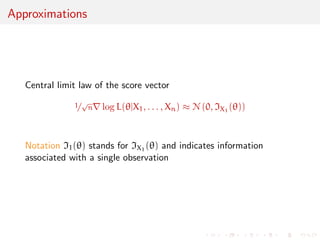
![Approximations
Back to the Kullback{Leibler divergence
D(0, ) =
Z
X
f(xj0) log f(xj0)=f(xj) dx
Using a second degree Taylor expansion
log f(xj) = log f(xj0) + ( - 0)Trlog f(xj0)
+
1
2
( - 0)TrrT log f(xj0)( - 0) + o(jj - 0 jj2)
approximation of divergence:
D(0, )
1
2
( - 0)TI(0)( - 0)
[Exercise: show this is exact in the normal case]](https://image.slidesharecdn.com/like-141026114245-conversion-gate02/85/Statistics-1-estimation-Chapter-3-likelihood-function-and-likelihood-estimation-50-320.jpg)
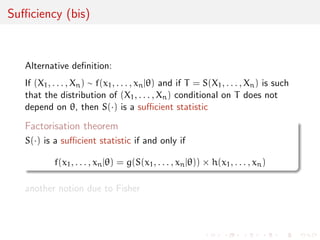
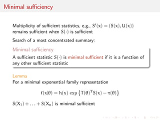
![Suciency
What if a transform of the sample
S(X1, . . . ,Xn)
contains all the information, i.e.
I(X1,...,Xn)() = IS(X1,...,Xn)()
uniformly in ?
In this case S() is called a sucient statistic [because it is
sucient to know the value of S(x1, . . . , xn) to get complete
information]
A statistic is an arbitrary transform of the data X1, . . . ,Xn](https://image.slidesharecdn.com/like-141026114245-conversion-gate02/85/Statistics-1-estimation-Chapter-3-likelihood-function-and-likelihood-estimation-52-320.jpg)
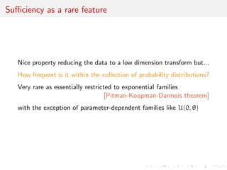
![Suciency as a rare feature
Nice property reducing the data to a low dimension transform but...
How frequent is it within the collection of probability distributions?
Very rare as essentially restricted to exponential families
[Pitman-Koopman-Darmois theorem]
with the exception of parameter-dependent families like U(0, )](https://image.slidesharecdn.com/like-141026114245-conversion-gate02/85/Statistics-1-estimation-Chapter-3-likelihood-function-and-likelihood-estimation-59-320.jpg)
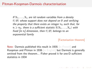
![xed [in n] dimension, then f(j) belongs to an
exponential family
[Factorisation theorem]
Note: Darmois published this result in 1935 [in French] and
Koopman and Pitman in 1936 [in English] but Darmois is generally
omitted from the theorem... Fisher proved it for one-D sucient
statistics in 1934](https://image.slidesharecdn.com/like-141026114245-conversion-gate02/85/Statistics-1-estimation-Chapter-3-likelihood-function-and-likelihood-estimation-61-320.jpg)
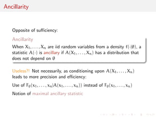
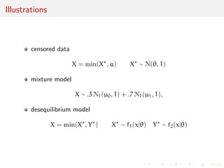
![Illustrations
1 If X1, . . . ,Xn
iid
U(0, ), A(X1, . . . ,Xn) = (X1, . . . ,Xn)=X(n)
is ancillary
2 If X1, . . . ,Xn
iid
N(, 2),
A(X1, . . . ,Xn) =
(X1P- Xn, . . . ,Xn - Xn n
i=1(Xi - Xn)2
is ancillary
3 If X1, . . . ,Xn
iid
f(xj), rank(X1, . . . ,Xn) is ancillary
x=rnorm(10)
rank(x)
[1] 7 4 1 5 2 6 8 9 10 3
[see, e.g., rank tests]](https://image.slidesharecdn.com/like-141026114245-conversion-gate02/85/Statistics-1-estimation-Chapter-3-likelihood-function-and-likelihood-estimation-64-320.jpg)
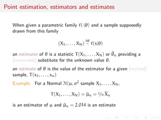
![Point estimation, estimators and estimates
When given a parametric family f(j) and a sample supposedly
drawn from this family
(X1, . . . ,XN)
iid
f(xj)
an estimator of is a statistic T(X1, . . . ,XN) or ^n providing a
[reasonable] substitute for the unknown value .
an estimate of is the value of the estimator for a given [realised]
sample, T(x1, . . . , xn)
Example: For a Normal N(, 2 sample X1, . . . ,XN,
T(X1, . . . ,XN) = ^n = 1=n Xn
is an estimator of and ^n = 2.014 is an estimate](https://image.slidesharecdn.com/like-141026114245-conversion-gate02/85/Statistics-1-estimation-Chapter-3-likelihood-function-and-likelihood-estimation-65-320.jpg)
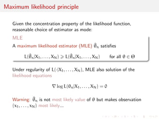
![Maximum likelihood invariance
Principle independent of parameterisation:
If = h() is a one-to-one transform of , then
^
MLE
n = h(^MLE
n )
[estimator of transform = transform of estimator]
By extension, if = h() is any transform of , then
^
MLE
n = h(^MLE
n )](https://image.slidesharecdn.com/like-141026114245-conversion-gate02/85/Statistics-1-estimation-Chapter-3-likelihood-function-and-likelihood-estimation-68-320.jpg)
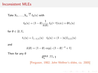
![nity of MLE's [or of solutions to likelihood
equations]
3
1
2 Case of x1, . . . , xn N(1 + 2, 1) [[and mixtures of normal]
3](https://image.slidesharecdn.com/like-141026114245-conversion-gate02/85/Statistics-1-estimation-Chapter-3-likelihood-function-and-likelihood-estimation-71-320.jpg)
![Unicity of MLE for exponential families
lemma
If f(j) is a minimal exponential family
f(xj) = h(x) exp
T()TS(x) - ()
with T() one-to-one and twice dierentiable over , if is open,
and if there is at least one solution to the likelihood equations,
then it is the unique MLE
Likelihood equation is equivalent to S(x) = E[S(x)]](https://image.slidesharecdn.com/like-141026114245-conversion-gate02/85/Statistics-1-estimation-Chapter-3-likelihood-function-and-likelihood-estimation-75-320.jpg)
![Unicity of MLE for exponential families
Likelihood equation is equivalent to S(x) = E[S(x)]
lemma
If is connected and open, and if `() is twice-dierentiable with
lim
!@
`() +1
and if H() = rrT`() is positive de](https://image.slidesharecdn.com/like-141026114245-conversion-gate02/85/Statistics-1-estimation-Chapter-3-likelihood-function-and-likelihood-estimation-76-320.jpg)
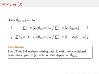

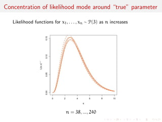
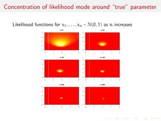
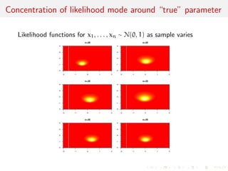
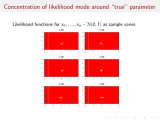
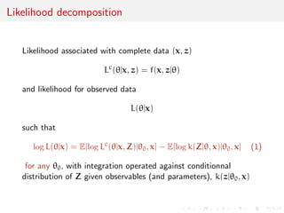
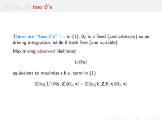
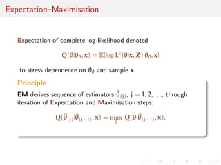
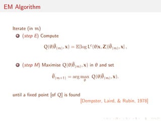
The document discusses likelihood functions and inference. It begins by defining the likelihood function as the function that gives the probability of observing a sample given a parameter value. The likelihood varies with the parameter, while the density function varies with the data. Maximum likelihood estimation chooses parameters that maximize the likelihood function. The score function is the gradient of the log-likelihood and has an expected value of zero at the true parameter value. The Fisher information matrix measures the curvature of the likelihood surface and provides information about the precision of parameter estimates. It relates to the concentration of likelihood functions around the true parameter value as sample size increases.