Download as PDF, PPTX


![An early entry
A standard issue in Bayesian inference is to approximate the
marginal likelihood (or evidence)
Ek =
Z
Θk
πk(ϑk)Lk(ϑk) dϑk,
aka the marginal likelihood.
[Jeffreys, 1939]](https://image.slidesharecdn.com/masterkl-220506133627-ac0e2786/85/CDT-22-slides-pdf-3-320.jpg)
![Bayes factor
For testing hypotheses H0 : ϑ ∈ Θ0 vs. Ha : ϑ 6∈ Θ0, under prior
π(Θ0)π0(ϑ) + π(Θc
0)π1(ϑ) ,
central quantity
B01 =
π(Θ0|x)
π(Θc
0|x)
π(Θ0)
π(Θc
0)
=
Z
Θ0
f(x|ϑ)π0(ϑ)dϑ
Z
Θc
0
f(x|ϑ)π1(ϑ)dϑ
[Kass Raftery, 1995, Jeffreys, 1939]](https://image.slidesharecdn.com/masterkl-220506133627-ac0e2786/85/CDT-22-slides-pdf-4-320.jpg)

![Forgetting and learning
Counterintuitive choice of importance function based on
mixtures
If ϑit ∼ $i(ϑ) (i = 1, . . . , I, t = 1, . . . , Ti)
Eπ[h(ϑ)] ≈
1
Ti
Ti
X
t=1
h(ϑit)
π(ϑit)
$i(ϑit)
replaced with
Eπ[h(ϑ)] ≈
I
X
i=1
Ti
X
t=1
h(ϑit)
π(ϑit)
PI
j=1 Tj$j(ϑit)
Preserves unbiasedness and brings stability (while forgetting
about original index)
[Geyer, 1991, unpublished; Owen Zhou, 2000]](https://image.slidesharecdn.com/masterkl-220506133627-ac0e2786/85/CDT-22-slides-pdf-6-320.jpg)


![Illustration
Special case when I = 2, c1 = 1, T1 = T2
−`(c2) =
T
X
t=1
log{1 + c2
e
$2(ϑ1t)/$1(ϑ1t)}
+
T
X
t=1
log{1 + $1(ϑ2t)/c2
e
$2(ϑ2t)}
tg=function(x)exp(-(x-5)**2/2)
pl=function(a)
sum(log(1+a*tg(x)/dnorm(x,0,3)))+sum(log(1+dnorm(y,0,3)/a/tg(y)))
nrm=matrix(0,3,1e2)
for(i in 1:3)
for(j in 1:1e2)
x=rnorm(10**(i+1),0,3)
y=rnorm(10**(i+1),5,1)
nrm[i,j]=optimise(pl,c(.01,1))](https://image.slidesharecdn.com/masterkl-220506133627-ac0e2786/85/CDT-22-slides-pdf-10-320.jpg)


![Bridge sampling
Approximation of Bayes factors (and other ratios of integrals)
Special case:
If
π1(ϑ1|x) ∝ π̃1(ϑ1|x)
π2(ϑ2|x) ∝ π̃2(ϑ2|x)
live on the same space (Θ1 = Θ2), then
B12 ≈
1
n
n
X
i=1
π̃1(ϑi|x)
π̃2(ϑi|x)
ϑi ∼ π2(ϑ|x)
[Bennett, 1976; Gelman Meng, 1998; Chen, Shao Ibrahim, 2000]](https://image.slidesharecdn.com/masterkl-220506133627-ac0e2786/85/CDT-22-slides-pdf-14-320.jpg)


![Optimal bridge sampling (2)
Reason:
Var(b
B12)
B2
12
≈
1
n1n2
R
π1(ϑ)π2(ϑ)[n1π1(ϑ) + n2π2(ϑ)]α(ϑ)2 dϑ
R
π1(ϑ)π2(ϑ)α(ϑ) dϑ
2
− 1
(by the δ method)
Drawback: Dependence on the unknown normalising constants
solved iteratively](https://image.slidesharecdn.com/masterkl-220506133627-ac0e2786/85/CDT-22-slides-pdf-19-320.jpg)
![Optimal bridge sampling (2)
Reason:
Var(b
B12)
B2
12
≈
1
n1n2
R
π1(ϑ)π2(ϑ)[n1π1(ϑ) + n2π2(ϑ)]α(ϑ)2 dϑ
R
π1(ϑ)π2(ϑ)α(ϑ) dϑ
2
− 1
(by the δ method)
Drawback: Dependence on the unknown normalising constants
solved iteratively](https://image.slidesharecdn.com/masterkl-220506133627-ac0e2786/85/CDT-22-slides-pdf-20-320.jpg)


![Mixtures as proposals
Design specific mixture for simulation purposes, with density
e
ϕ(ϑ) ∝ ω1π(ϑ)L(ϑ) + ϕ(ϑ) ,
where ϕ(ϑ) is arbitrary (but normalised)
Note: ω1 is not a probability weight
[Chopin Robert, 2011]](https://image.slidesharecdn.com/masterkl-220506133627-ac0e2786/85/CDT-22-slides-pdf-24-320.jpg)
![Mixtures as proposals
Design specific mixture for simulation purposes, with density
e
ϕ(ϑ) ∝ ω1π(ϑ)L(ϑ) + ϕ(ϑ) ,
where ϕ(ϑ) is arbitrary (but normalised)
Note: ω1 is not a probability weight
[Chopin Robert, 2011]](https://image.slidesharecdn.com/masterkl-220506133627-ac0e2786/85/CDT-22-slides-pdf-25-320.jpg)
![evidence approximation by mixtures
Rao-Blackwellised estimate
^
ξ =
1
T
T
X
t=1
ω1π(ϑ(t)
)L(ϑ(t)
)
ω1π(ϑ(t)
)L(ϑ(t)
) + ϕ(ϑ(t)
) ,
converges to ω1Z/{ω1Z + 1}
Deduce ^
Z from
ω1
^
Z/{ω1
^
Z + 1} = ^
ξ
Back to bridge sampling optimal estimate
[Chopin Robert, 2011]](https://image.slidesharecdn.com/masterkl-220506133627-ac0e2786/85/CDT-22-slides-pdf-26-320.jpg)
![Non-parametric MLE
“At first glance, the problem appears to be an exercise in
calculus or numerical analysis, and not amenable to statistical
formulation” Kong et al. (JRSS B, 2002)
I use of Fisher information
I non-parametric MLE based on
simulations
I comparison of sampling
schemes through variances
I Rao–Blackwellised
improvements by invariance
constraints [Meng, 2011, IRCEM]](https://image.slidesharecdn.com/masterkl-220506133627-ac0e2786/85/CDT-22-slides-pdf-27-320.jpg)
![Non-parametric MLE
“At first glance, the problem appears to be an exercise in
calculus or numerical analysis, and not amenable to statistical
formulation” Kong et al. (JRSS B, 2002)
I use of Fisher information
I non-parametric MLE based on
simulations
I comparison of sampling
schemes through variances
I Rao–Blackwellised
improvements by invariance
constraints [Meng, 2011, IRCEM]](https://image.slidesharecdn.com/masterkl-220506133627-ac0e2786/85/CDT-22-slides-pdf-28-320.jpg)

![NPMLE
Observing
Yij ∼ Fi(t) = c−1
i
Zt
−∞
ωi(x) dF(x)
with ωi known and F unknown
“Maximum likelihood estimate” defined by weighted empirical
cdf X
i,j
ωi(yij)p(yij)δyij
maximising in p Y
ij
c−1
i ωi(yij) p(yij)
Result such that
X
ij
^
c−1
r ωr(yij)
P
s ns^
c−1
s ωs(yij)
= 1
[Vardi, 1985]](https://image.slidesharecdn.com/masterkl-220506133627-ac0e2786/85/CDT-22-slides-pdf-31-320.jpg)
![NPMLE
Observing
Yij ∼ Fi(t) = c−1
i
Zt
−∞
ωi(x) dF(x)
with ωi known and F unknown
Result such that
X
ij
^
c−1
r ωr(yij)
P
s ns^
c−1
s ωs(yij)
= 1
[Vardi, 1985]
Bridge sampling estimator
X
ij
^
c−1
r ωr(yij)
P
s ns^
c−1
s ωs(yij)
= 1
[Gelman Meng, 1998; Tan, 2004]](https://image.slidesharecdn.com/masterkl-220506133627-ac0e2786/85/CDT-22-slides-pdf-32-320.jpg)
![end of the Series B 2002 discussion
“...essentially every Monte Carlo activity may be interpreted as
parameter estimation by maximum likelihood in a statistical
model. We do not claim that this point of view is necessary; nor
do we seek to establish a working principle from it.”
I restriction to discrete support measures [may be] suboptimal
[Ritov Bickel, 1990; Robins et al., 1997, 2000, 2003]
I group averaging versions in-between multiple mixture
estimators and quasi-Monte Carlo version
[Owen Zhou, 2000; Cornuet et al., 2012; Owen, 2003]
I statistical analogy provides at best narrative thread](https://image.slidesharecdn.com/masterkl-220506133627-ac0e2786/85/CDT-22-slides-pdf-33-320.jpg)


![Noise contrastive estimation
New estimation principle for parameterised and unnormalised
statistical models also based on nonlinear logistic regression
Case of parameterised model with density
p(x; α) =
p̃(x; α)
Z(α)
and untractable normalising constant Z(α)
Estimating Z(α) as extra parameter is impossible via maximum
likelihood methods
Use of estimation techniques bypassing the constant like
contrastive divergence (Hinton, 2002) and score matching
(Hyvärinen, 2005)
[Gutmann Hyvärinen, 2010]](https://image.slidesharecdn.com/masterkl-220506133627-ac0e2786/85/CDT-22-slides-pdf-37-320.jpg)
![Noise contrastive estimation
New estimation principle for parameterised and unnormalised
statistical models also based on nonlinear logistic regression
Case of parameterised model with density
p(x; α) =
p̃(x; α)
Z(α)
and untractable normalising constant Z(α)
Estimating Z(α) as extra parameter is impossible via maximum
likelihood methods
Use of estimation techniques bypassing the constant like
contrastive divergence (Hinton, 2002) and score matching
(Hyvärinen, 2005)
[Gutmann Hyvärinen, 2010]](https://image.slidesharecdn.com/masterkl-220506133627-ac0e2786/85/CDT-22-slides-pdf-38-320.jpg)
![Noise contrastive estimation
New estimation principle for parameterised and unnormalised
statistical models also based on nonlinear logistic regression
Case of parameterised model with density
p(x; α) =
p̃(x; α)
Z(α)
and untractable normalising constant Z(α)
Estimating Z(α) as extra parameter is impossible via maximum
likelihood methods
Use of estimation techniques bypassing the constant like
contrastive divergence (Hinton, 2002) and score matching
(Hyvärinen, 2005)
[Gutmann Hyvärinen, 2010]](https://image.slidesharecdn.com/masterkl-220506133627-ac0e2786/85/CDT-22-slides-pdf-39-320.jpg)


![NCE consistency
Objective function that converges (in T) to
J(ϑ) = E [log h(x; ϑ) + log{1 − h(y; ϑ)}]
Defining f(·) = log p(·; ϑ) and
J̃(f) = Ep [log r(f(x) − log q(x)) + log{1 − r(f(y) − log q(y))}]](https://image.slidesharecdn.com/masterkl-220506133627-ac0e2786/85/CDT-22-slides-pdf-42-320.jpg)
![NCE consistency
Objective function that converges (in T) to
J(ϑ) = E [log h(x; ϑ) + log{1 − h(y; ϑ)}]
Defining f(·) = log p(·; ϑ) and
J̃(f) = Ep [log r(f(x) − log q(x)) + log{1 − r(f(y) − log q(y))}]
Assuming q(·) positive everywhere,
I J̃(·) attains its maximum at f?(·) = log p(·) true distribution
I maximization performed without any normalisation
constraint](https://image.slidesharecdn.com/masterkl-220506133627-ac0e2786/85/CDT-22-slides-pdf-43-320.jpg)
![NCE consistency
Objective function that converges (in T) to
J(ϑ) = E [log h(x; ϑ) + log{1 − h(y; ϑ)}]
Defining f(·) = log p(·; ϑ) and
J̃(f) = Ep [log r(f(x) − log q(x)) + log{1 − r(f(y) − log q(y))}]
Under regularity condition, assuming the true distribution
belongs to parametric family, the solution
^
ϑT = arg max
ϑ
`(ϑ; x, y) (1)
converges to true ϑ
Consequence: log-normalisation constant consistently
estimated by maximizing (??)](https://image.slidesharecdn.com/masterkl-220506133627-ac0e2786/85/CDT-22-slides-pdf-44-320.jpg)
![Convergence of noise contrastive estimation
Opposition of Monte Carlo MLE à la Geyer (1994, JASA)
L = 1/n
n
X
i=1
log p̃(xi; ϑ)
p̃(xi; ϑ0
)
− log
1/m
m
X
j=1
p̃(zi; ϑ)
p̃(zi; ϑ0
)
| {z }
≈Z(ϑ0)/Z(ϑ)
x1, . . . , xn ∼ p∗
z1, . . . , zm ∼ p(z; ϑ0
)
[Riou-Durand Chopin, 2018]](https://image.slidesharecdn.com/masterkl-220506133627-ac0e2786/85/CDT-22-slides-pdf-45-320.jpg)
![Convergence of noise contrastive estimation
and of noise contrastive estimation à la Gutmann and
Hyvärinen (2012)
L(ϑ, ν) = 1/n
n
X
i=1
log qϑ,ν(xi) + 1/m
m
X
i=1
log[1 − qϑ,ν(zi)]m/n
log
qϑ,ν(z)
1 − qϑ,ν(z)
= log
p̃(xi; ϑ)
p̃(xi; ϑ0)
+ ν + log n/m
x1, . . . , xn ∼ p∗
z1, . . . , zm ∼ p(z; ϑ0
)
[Riou-Durand Chopin, 2018]](https://image.slidesharecdn.com/masterkl-220506133627-ac0e2786/85/CDT-22-slides-pdf-46-320.jpg)

![NCE consistency
Under mild assumptions, almost surely
^
ξMCMLE
n,m
m→∞
−→ ^
ξn
and
^
ξNCE
n,m
m→∞
−→ ^
ξn
the maximum likelihood estimator associated with
x1, . . . , xn ∼ p(·; ϑ)
and
e−^
ν
=
Z(^
ϑ)
Z(ϑ0)
[Geyer, 1994; Riou-Durand Chopin, 2018]](https://image.slidesharecdn.com/masterkl-220506133627-ac0e2786/85/CDT-22-slides-pdf-48-320.jpg)
![NCE asymptotics
Under less mild assumptions (more robust for NCE),
asymptotic normality of both NCE and MC-MLE estimates as
n −→ +∞ m/n −→ τ
√
n(^
ξMCMLE
n,m − ξ∗
) ≈ Nd(0, ΣMCMLE
)
and √
n(^
ξNCE
n,m − ξ∗
) ≈ Nd(0, ΣNCE
)
with important ordering
ΣMCMLE
ΣNCE
showing that NCE dominates MCMLE in terms of mean square
error (for iid simulations)
[Geyer, 1994; Riou-Durand Chopin, 2018]](https://image.slidesharecdn.com/masterkl-220506133627-ac0e2786/85/CDT-22-slides-pdf-49-320.jpg)
![NCE asymptotics
Under less mild assumptions (more robust for NCE),
asymptotic normality of both NCE and MC-MLE estimates as
n −→ +∞ m/n −→ τ
√
n(^
ξMCMLE
n,m − ξ∗
) ≈ Nd(0, ΣMCMLE
)
and √
n(^
ξNCE
n,m − ξ∗
) ≈ Nd(0, ΣNCE
)
with important ordering except when ϑ0 = ϑ∗
ΣMCMLE
= ΣNCE
= (1 + τ−1
)ΣRMLNCE
[Geyer, 1994; Riou-Durand Chopin, 2018]](https://image.slidesharecdn.com/masterkl-220506133627-ac0e2786/85/CDT-22-slides-pdf-50-320.jpg)
![NCE asymptotics
[Riou-Durand Chopin, 2018]](https://image.slidesharecdn.com/masterkl-220506133627-ac0e2786/85/CDT-22-slides-pdf-51-320.jpg)
![NCE contrast distribution
Choice of q(·) free but
I easy to sample from
I must allows for analytical expression of its log-pdf
I must be close to true density p(·), so that mean squared
error E[|^
ϑT − ϑ?|2] small
Learning an approximation ^
q to p(·), for instance via
normalising flows
[Tabak and Turner, 2013; Jia Seljiak, 2019]](https://image.slidesharecdn.com/masterkl-220506133627-ac0e2786/85/CDT-22-slides-pdf-52-320.jpg)
![NCE contrast distribution
Choice of q(·) free but
I easy to sample from
I must allows for analytical expression of its log-pdf
I must be close to true density p(·), so that mean squared
error E[|^
ϑT − ϑ?|2] small
Learning an approximation ^
q to p(·), for instance via
normalising flows
[Tabak and Turner, 2013; Jia Seljiak, 2019]](https://image.slidesharecdn.com/masterkl-220506133627-ac0e2786/85/CDT-22-slides-pdf-53-320.jpg)
![NCE contrast distribution
Choice of q(·) free but
I easy to sample from
I must allows for analytical expression of its log-pdf
I must be close to true density p(·), so that mean squared
error E[|^
ϑT − ϑ?|2] small
Learning an approximation ^
q to p(·), for instance via
normalising flows
[Tabak and Turner, 2013; Jia Seljiak, 2019]](https://image.slidesharecdn.com/masterkl-220506133627-ac0e2786/85/CDT-22-slides-pdf-54-320.jpg)
![Density estimation by normalising flows
“A normalizing flow describes the transformation of a
probability density through a sequence of invertible map-
pings. By repeatedly applying the rule for change of
variables, the initial density ‘flows’ through the sequence
of invertible mappings. At the end of this sequence we
obtain a valid probability distribution and hence this type
of flow is referred to as a normalizing flow.”
[Rezende Mohammed, 2015; Papamakarios et al., 2021]](https://image.slidesharecdn.com/masterkl-220506133627-ac0e2786/85/CDT-22-slides-pdf-55-320.jpg)
![Density estimation by normalising flows
Based on invertible and 2×differentiable transforms
(diffeomorphisms) gi(·) = g(·; ηi) of a standard distribution ϕ(·)
Representation
z = g1 ◦ · · · ◦ gp(x) x ∼ ϕ(x)
Density of z by Jacobian transform
ϕ(x(z)) × detJg1◦···◦gp (z) = ϕ(x(z))
Y
i
|dgi/dzi−1|−1
where zi = gi(zi−1)
Flow defined as x − z1 − . . . − zp = z
[Rezende Mohammed, 2015; Papamakarios et al., 2021]](https://image.slidesharecdn.com/masterkl-220506133627-ac0e2786/85/CDT-22-slides-pdf-56-320.jpg)
![Density estimation by normalising flows
Flow defined as x − z1 − . . . − zp = z
Density of z by Jacobian transform
ϕ(x(z)) × detJg1◦···◦gp (z) = ϕ(x(z))
Y
i
|dgi/dzi−1|−1
where zi = gi(zi−1)
Composition of transforms
(g1 ◦ g2)−1
= g−1
2 ◦ g−1
1 (2)
detJg1◦g2
(u) = detJg1
(g2(u)) × detJg2
(u) (3)
[Rezende Mohammed, 2015; Papamakarios et al., 2021]](https://image.slidesharecdn.com/masterkl-220506133627-ac0e2786/85/CDT-22-slides-pdf-57-320.jpg)
![Density estimation by normalising flows
Flow defined as x, z1, . . . , zp = z
Density of z by Jacobian transform
ϕ(x(z)) × detJg1◦···◦gp (z) = ϕ(x(z))
Y
i
|dgi/dzi−1|−1
where zi = gi(zi−1)
[Rezende Mohammed, 2015; Papamakarios et al., 2021]](https://image.slidesharecdn.com/masterkl-220506133627-ac0e2786/85/CDT-22-slides-pdf-58-320.jpg)


![= |det(Id + uψ(z)0
)| = |1 + u0
ψ(z)|
[Rezende Mohammed, 2015]](https://image.slidesharecdn.com/masterkl-220506133627-ac0e2786/85/CDT-22-slides-pdf-68-320.jpg)
![Invertible linear-time transformations
Family of transformations
g(z) = z + uh(w0
z + b), u, w ∈ Rd
, b ∈ R
with h smooth element-wise non-linearity transform, with
derivative h0
Density q(z) obtained by transforming initial density ϕ(z)
through sequence of maps gi, i.e.
z = gp ◦ · · · ◦ g1(x)
and
log q(z) = log ϕ(x) −
p
X
k=1
log |1 + u0
ψk(zk−1)|
[Rezende Mohammed, 2015]](https://image.slidesharecdn.com/masterkl-220506133627-ac0e2786/85/CDT-22-slides-pdf-69-320.jpg)
![General theory of normalising flows
”Normalizing flows provide a general mechanism for
defining expressive probability distributions, only requir-
ing the specification of a (usually simple) base distribu-
tion and a series of bijective transformations.”
T(u; ψ) = gp(gp−1(. . . g1(u; η1) . . . ; ηp−1); ηp)
[Papamakarios et al., 2021]](https://image.slidesharecdn.com/masterkl-220506133627-ac0e2786/85/CDT-22-slides-pdf-70-320.jpg)
![General theory of normalising flows
“...how expressive are flow-based models? Can they rep-
resent any distribution p(x), even if the base distribution
is restricted to be simple? We show that this universal
representation is possible under reasonable conditions
on p(x).”
Obvious when considering the inverse conditional cdf
transforms, assuming differentiability
[Papamakarios et al., 2021]](https://image.slidesharecdn.com/masterkl-220506133627-ac0e2786/85/CDT-22-slides-pdf-71-320.jpg)
![General theory of normalising flows
[Hyvärinen Pajunen (1999)]
I Write
px(x) =
d
Y
i=1
p(xi|xi)
I define
zi = Fi(xi, xi) = P(Xi ≤ xi|xi)
I deduce that
det JF(x) = p(x)
I conclude that pz(z) = 1 Uniform on (0, 1)d
[Papamakarios et al., 2021]](https://image.slidesharecdn.com/masterkl-220506133627-ac0e2786/85/CDT-22-slides-pdf-72-320.jpg)
![General theory of normalising flows
“Minimizing the Monte Carlo approximation of the
Kullback–Leibler divergence [between the true and the
model densities] is equivalent to fitting the flow-based
model to the sample by maximum likelihood estimation.”
MLEstimate flow-based model parameters by
arg max
ψ
n
X
i=1
log{ϕ(T−1
(xi; ψ))} − log |det{JT−1 (xi; ψ)}|
Note possible use of reverse Kullback–Leibler divergence when
learning an approximation (VA, IS, ABC) to a known [up to a
constant] target p(x)
[Papamakarios et al., 2021]](https://image.slidesharecdn.com/masterkl-220506133627-ac0e2786/85/CDT-22-slides-pdf-73-320.jpg)


![Table 1: Multiple choices for
I transformer τ(·; ϕ)
I conditioner c(·) (neural network)
[Papamakarios et al., 2021]](https://image.slidesharecdn.com/masterkl-220506133627-ac0e2786/85/CDT-22-slides-pdf-95-320.jpg)
![Practical considerations
“Implementing a flow often amounts to composing as
many transformations as computation and memory will
allow. Working with such deep flows introduces addi-
tional challenges of a practical nature.”
I the more the merrier?!
I batch normalisation for maintaining stable gradients
(between layers)
I fighting curse of dimension (“evaluating T incurs an
increasing computational cost as dimensionality grows”)
with multiscale architecture (clamping: component-wise
stopping rules)
[Papamakarios et al., 2021]](https://image.slidesharecdn.com/masterkl-220506133627-ac0e2786/85/CDT-22-slides-pdf-96-320.jpg)
![Practical considerations
“Implementing a flow often amounts to composing as
many transformations as computation and memory will
allow. Working with such deep flows introduces addi-
tional challenges of a practical nature.”
I the more the merrier?!
I batch normalisation for maintaining stable gradients
(between layers)
I “...early work on flow precursors dismissed the
autoregressive approach as prohibitively expensive”
addressed by sharing parameters within conditioners ci(·)
[Papamakarios et al., 2021]](https://image.slidesharecdn.com/masterkl-220506133627-ac0e2786/85/CDT-22-slides-pdf-97-320.jpg)
![Applications
“Normalizing flows have two primitive operations: den-
sity calculation and sampling. In turn, flows are effec-
tive in any application requiring a probabilistic model
with either of those capabilities.”
I density estimation [speed of convergence?]
I proxy generative model
I importance sampling for integration by minimising distance
to integrand or IS variance [finite?]
I MCMC flow substitute for HMC
[Papamakarios et al., 2021]](https://image.slidesharecdn.com/masterkl-220506133627-ac0e2786/85/CDT-22-slides-pdf-98-320.jpg)
![Applications
“Normalizing flows have two primitive operations: den-
sity calculation and sampling. In turn, flows are effec-
tive in any application requiring a probabilistic model
with either of those capabilities.”
I optimised reparameterisation of target for MCMC [exact?]
I variational approximation by maximising evidence lower
bound (ELBO) to posterior on parameter η = T(u, ϕ)
n
X
i=1
log p(xobs
, T(ui; ϕ))
| {z }
joint
+ log |detJT (ui; ϕ)|
I substitutes for likelihood-free inference on either π(η|xobs)
or p(xobs|η)
[Papamakarios et al., 2021]](https://image.slidesharecdn.com/masterkl-220506133627-ac0e2786/85/CDT-22-slides-pdf-99-320.jpg)
![A[nother] revolution in machine learning?
“One area where neural networks are being actively de-
veloped is density estimation in high dimensions: given
a set of points x ∼ p(x), the goal is to estimate the
probability density p(·). As there are no explicit la-
bels, this is usually considered an unsupervised learning
task. We have already discussed that classical methods
based for instance on histograms or kernel density esti-
mation do not scale well to high-dimensional data. In
this regime, density estimation techniques based on neu-
ral networks are becoming more and more popular. One
class of these neural density estimation techniques are
normalizing flows.”
[Cranmer et al., PNAS, 2020]](https://image.slidesharecdn.com/masterkl-220506133627-ac0e2786/85/CDT-22-slides-pdf-100-320.jpg)
![Crucially lacking
No connection with statistical density estimation, with no
general study of convergence (in training sample size) to the
true density
...or in evaluating approximation error (as in ABC)
[Kobyzev et al., 2019; Papamakarios et al., 2021]](https://image.slidesharecdn.com/masterkl-220506133627-ac0e2786/85/CDT-22-slides-pdf-101-320.jpg)
![Reconnecting with Geyer (1994)
“...neural networks can be trained to learn the likelihood
ratio function p(x|ϑ0)/p(x|ϑ1) or p(x|ϑ0)/p(x), where in
the latter case the denominator is given by a marginal
model integrated over a proposal or the prior (...) The
key idea is closely related to the discriminator network
in GANs mentioned above: a classifier is trained us-
ing supervised learning to discriminate two sets of data,
though in this case both sets come from the simulator
and are generated for different parameter points ϑ0 and
ϑ1. The classifier output function can be converted into
an approximation of the likelihood ratio between ϑ0 and
ϑ1! This manifestation of the Neyman-Pearson lemma
in a machine learning setting is often called the likeli-
hood ratio trick.”
[Cranmer et al., PNAS, 2020]](https://image.slidesharecdn.com/masterkl-220506133627-ac0e2786/85/CDT-22-slides-pdf-102-320.jpg)
![A comparison with MLE
[Guttmann Hyvärinen, 2012]](https://image.slidesharecdn.com/masterkl-220506133627-ac0e2786/85/CDT-22-slides-pdf-103-320.jpg)
![A comparison with MLE
[Guttmann Hyvärinen, 2012]](https://image.slidesharecdn.com/masterkl-220506133627-ac0e2786/85/CDT-22-slides-pdf-104-320.jpg)
![A comparison with MLE
[Guttmann Hyvärinen, 2012]](https://image.slidesharecdn.com/masterkl-220506133627-ac0e2786/85/CDT-22-slides-pdf-105-320.jpg)


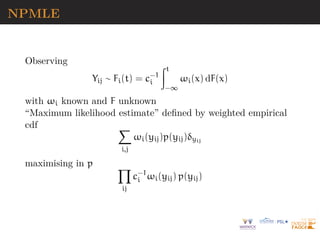
![Likelihood complexity
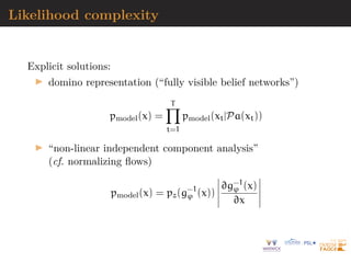
Implicit solutions involving sampling from the model pmodel
without computing density
I ABC algorithms for MLE derivation
[Piccini Anderson, 2017]
I generative stochastic networks
[Bengio et al., 2014]
I generative adversarial networks (GANs)
[Goodfellow et al., 2014]](https://image.slidesharecdn.com/masterkl-220506133627-ac0e2786/85/CDT-22-slides-pdf-152-320.jpg)

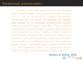
![Variational autoencoders
“... provide a principled framework for learning deep
latent-variable models and corresponding inference mod-
els (...) can be viewed as two coupled, but indepen-
dently parameterized models: the encoder or recogni-
tion model, and the decoder or generative model.
These two models support each other. The recognition
model delivers to the generative model an approximation
to its posterior over latent random variables, which it
needs to update its parameters inside an iteration of “ex-
pectation maximization” learning. Reversely, the gener-
ative model is a scaffolding of sorts for the recognition
model to learn meaningful representations of the data
(...) The recognition model is the approximate inverse
of the generative model according to Bayes rule.”
[Kingma Welling, 2019]](https://image.slidesharecdn.com/masterkl-220506133627-ac0e2786/85/CDT-22-slides-pdf-154-320.jpg)
![Autoencoders
“An autoencoder is a neural network that is trained to
attempt to copy its input x to its output r = g(h) via
a hidden layer h = f(x) (...) [they] are designed to be
unable to copy perfectly”
I undercomplete autoencoders (with dim(h) dim(x))
I regularised autoencoders, with objective
L(x, g ◦ f(x)) + Ω(h)
where penalty akin to log-prior
I denoising autoencoders (learning x on noisy version x̃ of x)
I stochastic autoencoders (learning pdecode(x|h) for a given
pencode(h|x) w/o compatibility)
[Goodfellow et al., 2016, p.496]](https://image.slidesharecdn.com/masterkl-220506133627-ac0e2786/85/CDT-22-slides-pdf-155-320.jpg)

![Variational autoencoders (VAEs)
“The key idea behind the variational autoencoder is to
attempt to sample values of Z that are likely to have
produced X = x, and compute p(x) just from those.”
Representation of (marginal) likelihood pϑ(x) based on latent
variable z
pϑ(x) =
Z
pϑ(x|z)pϑ(z) dz
Machine-learning usually preoccupied only by maximising pϑ(x)
(in ϑ) by simulating z efficiently (i.e., not from the prior)
log pϑ(x) − D[pϑ(·)||pϑ(·|x)] = Epϑ
[log pϑ(x|Z)] − D[qϕ(·)||pϑ(·)]
[Kingma Welling, 2019]](https://image.slidesharecdn.com/masterkl-220506133627-ac0e2786/85/CDT-22-slides-pdf-157-320.jpg)
![Variational autoencoders (VAEs)
“The key idea behind the variational autoencoder is to
attempt to sample values of Z that are likely to have
produced X = x, and compute p(x) just from those.”
Representation of (marginal) likelihood pϑ(x) based on latent
variable z
pϑ(x) =
Z
pϑ(x|z)pϑ(z) dz
Machine-learning usually preoccupied only by maximising pϑ(x)
(in ϑ) by simulating z efficiently (i.e., not from the prior)
log pϑ(x)−D[qϕ(·|x)||pϑ(·|x)] = Eqϕ(·|x)[log pϑ(x|Z)]−D[qϕ(·|x)||pϑ(·)]
since x is fixed (Bayesian analogy)
[Kingma Welling, 2019]](https://image.slidesharecdn.com/masterkl-220506133627-ac0e2786/85/CDT-22-slides-pdf-158-320.jpg)
![Variational autoencoders (VAEs)
[Kingma Welling, 2019]](https://image.slidesharecdn.com/masterkl-220506133627-ac0e2786/85/CDT-22-slides-pdf-159-320.jpg)
![Variational autoencoders (VAEs)
log pϑ(x)−D[qϕ(·|x)||pϑ(·|x)] = Eqϕ(·|x)[log pϑ(x|Z)]−D[qϕ(·|x)||pϑ(·)]
I lhs is quantity to maximize (plus error term, small for good
approximation qϕ, or regularisation)
I rhs can be optimised by stochastic gradient descent when
qϕ manageable
I link with autoencoder, as qϕ(z|x) “encoding” x into z, and
pϑ(x|z) “decoding” z to reconstruct x
[Doersch, 2021]](https://image.slidesharecdn.com/masterkl-220506133627-ac0e2786/85/CDT-22-slides-pdf-160-320.jpg)
![Variational autoencoders (VAEs)
log pϑ(x)−D[qϕ(·|x)||pϑ(·|x)] = Eqϕ(·|x)[log pϑ(x|Z)]−D[qϕ(·|x)||pϑ(·)]
I lhs is quantity to maximize (plus error term, small for good
approximation qϕ, or regularisation)
I rhs can be optimised by stochastic gradient descent when
qϕ manageable
I link with autoencoder, as qϕ(z|x) “encoding” x into z, and
pϑ(x|z) “decoding” z to reconstruct x
[Doersch, 2021]](https://image.slidesharecdn.com/masterkl-220506133627-ac0e2786/85/CDT-22-slides-pdf-161-320.jpg)
![Variational autoencoders (VAEs)
“One major division in machine learning is generative
versus discriminative modeling (...) To turn a genera-
tive model into a discriminator we need Bayes rule.”
Representation of (marginal) likelihood pϑ(x) based on latent
variable z
Variational approximation qϕ(z|x) (also called encoder) to
posterior distribution on latent variable z, pϑ(z|x), associated
with conditional distribution pϑ(x|z) (also called decoder)
Example: qϕ(z|x) Normal distribution Nd(µ(x), Σ(x)) with
I (µ(x), Σ(x)) estimated by deep neural network
I (µ(x), Σ(x)) estimated by ABC (synthetic likelihood)
[Kingma Welling, 2014]](https://image.slidesharecdn.com/masterkl-220506133627-ac0e2786/85/CDT-22-slides-pdf-162-320.jpg)
![Variational autoencoders (VAEs)
“One major division in machine learning is generative
versus discriminative modeling (...) To turn a genera-
tive model into a discriminator we need Bayes rule.”
Representation of (marginal) likelihood pϑ(x) based on latent
variable z
Variational approximation qϕ(z|x) (also called encoder) to
posterior distribution on latent variable z, pϑ(z|x), associated
with conditional distribution pϑ(x|z) (also called decoder)
Example: qϕ(z|x) Normal distribution Nd(µ(x), Σ(x)) with
I (µ(x), Σ(x)) estimated by deep neural network
I (µ(x), Σ(x)) estimated by ABC (synthetic likelihood)
[Kingma Welling, 2014]](https://image.slidesharecdn.com/masterkl-220506133627-ac0e2786/85/CDT-22-slides-pdf-163-320.jpg)
![ELBO objective
Since
log pϑ(x) = Eqϕ(z|x)[log pϑ(x)]
= Eqϕ(z|x)[log
pϑ(x, z)
pϑ(z|x)
]
= Eqϕ(z|x)[log
pϑ(x, z)
qϕ(z|x)
] + Eqϕ(z|x)[log
qϕ(x, z)
pϑ(z|x)
]
| {z }
KL≥0
evidence lower bound (ELBO) defined by
Lϑ,ϕ(x) = Eqϕ(z|x)[log pϑ(x, z)] − Eqϕ(z|x)[log qϕ(z|x)]
and used as objective function to be maximised in (ϑ, ϕ)](https://image.slidesharecdn.com/masterkl-220506133627-ac0e2786/85/CDT-22-slides-pdf-164-320.jpg)
![ELBO maximisation
Stochastic gradient step, one parameter at a time
In iid settings
Lϑ,ϕ(x) =
n
X
i=1
Lϑ,ϕ(xi)
and
∇ϑLϑ,ϕ(xi) = Eqϕ(z|xi)[∇ϑ log pϑ(xi, z)] ≈ ∇ϑ log pϑ(x, z̃(xi))
for one simulation z̃(xi) ∼ qϕ(z|xi)
but ∇ϕLϑ,ϕ(xi) more difficult to compute](https://image.slidesharecdn.com/masterkl-220506133627-ac0e2786/85/CDT-22-slides-pdf-165-320.jpg)
![ELBO maximisation
Stochastic gradient step, one parameter at a time
In iid settings
Lϑ,ϕ(x) =
n
X
i=1
Lϑ,ϕ(xi)
and
∇ϑLϑ,ϕ(xi) = Eqϕ(z|xi)[∇ϑ log pϑ(xi, z)] ≈ ∇ϑ log pϑ(x, z̃(xi))
for one simulation z̃(xi) ∼ qϕ(z|xi)
but ∇ϕLϑ,ϕ(xi) more difficult to compute](https://image.slidesharecdn.com/masterkl-220506133627-ac0e2786/85/CDT-22-slides-pdf-166-320.jpg)
![ELBO maximisation (2)
Reparameterisation (form of normalising flow)
If z = g(x, ϕ, ε) ∼ qϕ(z|x) when ε ∼ r(ε),
Eqϕ(z|xi)[h(Z)] = Er[h(g(x, ϕ, ε))]
and
∇ϕEqϕ(z|xi)[h(Z)] = ∇ϕEr[h ◦ g(x, ϕ, ε)]
= Er[∇ϕh ◦ g(x, ϕ, ε)]
≈ ∇ϕh ◦ g(x, ϕ, ε̃)
for one simulation ε̃ ∼ r
[Kingma Welling, 2014]](https://image.slidesharecdn.com/masterkl-220506133627-ac0e2786/85/CDT-22-slides-pdf-167-320.jpg)
![ELBO maximisation (2)
Reparameterisation (form of normalising flow)
If z = g(x, ϕ, ε) ∼ qϕ(z|x) when ε ∼ r(ε),
Eqϕ(z|xi)[h(Z)] = Er[h(g(x, ϕ, ε))]
leading to unbiased estimator of gradient of ELBO
∇ϑ,ϕ {log pϑ(x, g(x, ϕ, ε)) − log qϕ(g(x, ϕ, ε)|x)}
[Kingma Welling, 2014]](https://image.slidesharecdn.com/masterkl-220506133627-ac0e2786/85/CDT-22-slides-pdf-168-320.jpg)
![ELBO maximisation (2)
Reparameterisation (form of normalising flow)
If z = g(x, ϕ, ε) ∼ qϕ(z|x) when ε ∼ r(ε),
Eqϕ(z|xi)[h(Z)] = Er[h(g(x, ϕ, ε))]
leading to unbiased estimator of gradient of ELBO
∇ϑ,ϕ](https://image.slidesharecdn.com/masterkl-220506133627-ac0e2786/85/CDT-22-slides-pdf-169-320.jpg)


![[Kingma Welling, 2014]](https://image.slidesharecdn.com/masterkl-220506133627-ac0e2786/85/CDT-22-slides-pdf-178-320.jpg)


![Generative adversarial networks (GANs)
“Generative adversarial networks (GANs) provide an
algorithmic framework for constructing generative mod-
els with several appealing properties:
– they do not require a likelihood function to be specified,
only a generating procedure;
– they provide samples that are sharp and compelling;
– they allow us to harness our knowledge of building
highly accurate neural network classifiers.”
[Mohamed Lakshminarayanan, 2016]](https://image.slidesharecdn.com/masterkl-220506133627-ac0e2786/85/CDT-22-slides-pdf-182-320.jpg)
![Implicit generative models
Representation of random variables as
x = Gϑ(z) z ∼ µ(z)
where µ(·) reference distribution and Gϑ multi-layered and
highly non-linear transform (as, e.g., in normalizing flows)
I more general and flexible than “prescriptive” if implicit
(black box)
I connected with pseudo-random variable generation
I call for likelihood-free inference on ϑ
[Mohamed Lakshminarayanan, 2016]](https://image.slidesharecdn.com/masterkl-220506133627-ac0e2786/85/CDT-22-slides-pdf-183-320.jpg)
![Implicit generative models
Representation of random variables as
x = Gϑ(z) z ∼ µ(z)
where µ(·) reference distribution and Gϑ multi-layered and
highly non-linear transform (as, e.g., in normalizing flows)
I more general and flexible than “prescriptive” if implicit
(black box)
I connected with pseudo-random variable generation
I call for likelihood-free inference on ϑ
[Mohamed Lakshminarayanan, 2016]](https://image.slidesharecdn.com/masterkl-220506133627-ac0e2786/85/CDT-22-slides-pdf-184-320.jpg)


![The ABC method
Bayesian setting: target is π(ϑ)f(x|ϑ)
When likelihood f(x|ϑ) not in closed form, likelihood-free
rejection technique:
ABC algorithm
For an observation y ∼ f(y|ϑ), under the prior π(ϑ), keep jointly
simulating
ϑ0
∼ π(ϑ) , z ∼ f(z|ϑ0
) ,
until the auxiliary variable z is equal to the observed value,
z = y.
[Tavaré et al., 1997]](https://image.slidesharecdn.com/masterkl-220506133627-ac0e2786/85/CDT-22-slides-pdf-187-320.jpg)
![The ABC method
Bayesian setting: target is π(ϑ)f(x|ϑ)
When likelihood f(x|ϑ) not in closed form, likelihood-free
rejection technique:
ABC algorithm
For an observation y ∼ f(y|ϑ), under the prior π(ϑ), keep jointly
simulating
ϑ0
∼ π(ϑ) , z ∼ f(z|ϑ0
) ,
until the auxiliary variable z is equal to the observed value,
z = y.
[Tavaré et al., 1997]](https://image.slidesharecdn.com/masterkl-220506133627-ac0e2786/85/CDT-22-slides-pdf-188-320.jpg)
![The ABC method
Bayesian setting: target is π(ϑ)f(x|ϑ)
When likelihood f(x|ϑ) not in closed form, likelihood-free
rejection technique:
ABC algorithm
For an observation y ∼ f(y|ϑ), under the prior π(ϑ), keep jointly
simulating
ϑ0
∼ π(ϑ) , z ∼ f(z|ϑ0
) ,
until the auxiliary variable z is equal to the observed value,
z = y.
[Tavaré et al., 1997]](https://image.slidesharecdn.com/masterkl-220506133627-ac0e2786/85/CDT-22-slides-pdf-189-320.jpg)
![Why does it work?!
The proof is trivial:
f(ϑi) ∝
X
z∈D
π(ϑi)f(z|ϑi)Iy(z)
∝ π(ϑi)f(y|ϑi)
= π(ϑi|y) .
[Accept–Reject 101]](https://image.slidesharecdn.com/masterkl-220506133627-ac0e2786/85/CDT-22-slides-pdf-190-320.jpg)
![ABC as A...pproximative
When y is a continuous random variable, equality z = y is
replaced with a tolerance condition,
ρ{η(z), η(y)} ≤ ε
where ρ is a distance and η(y) defines a (not necessarily
sufficient) statistic
Output distributed from
π(ϑ) Pϑ{ρ(y, z) ε} ∝ π(ϑ|ρ(η(y), η(z)) ε)
[Pritchard et al., 1999]](https://image.slidesharecdn.com/masterkl-220506133627-ac0e2786/85/CDT-22-slides-pdf-191-320.jpg)
![ABC as A...pproximative
When y is a continuous random variable, equality z = y is
replaced with a tolerance condition,
ρ{η(z), η(y)} ≤ ε
where ρ is a distance and η(y) defines a (not necessarily
sufficient) statistic
Output distributed from
π(ϑ) Pϑ{ρ(y, z) ε} ∝ π(ϑ|ρ(η(y), η(z)) ε)
[Pritchard et al., 1999]](https://image.slidesharecdn.com/masterkl-220506133627-ac0e2786/85/CDT-22-slides-pdf-192-320.jpg)


![MA example
Back to the MA(2) model
xt = εt +
2
X
i=1
ϑiεt−i
Simple prior: uniform over the inverse [real and complex] roots
in
Q(u) = 1 −
2
X
i=1
ϑiui
under identifiability conditions](https://image.slidesharecdn.com/masterkl-220506133627-ac0e2786/85/CDT-22-slides-pdf-195-320.jpg)


![Occurence of simulation in Econometrics
Simulation–based techniques in Econometrics
I Simulated method of moments
I Method of simulated moments
I Simulated pseudo-maximum-likelihood
I Indirect inference
[Gouriéroux Monfort, 1996]](https://image.slidesharecdn.com/masterkl-220506133627-ac0e2786/85/CDT-22-slides-pdf-202-320.jpg)


![Indirect inference
Minimise (in ϑ) the distance between estimators ^
β based on
pseudo-models for genuine observations and for observations
simulated under the true model and the parameter ϑ.
[Gouriéroux, Monfort, Renault, 1993;
Smith, 1993; Gallant Tauchen, 1996]](https://image.slidesharecdn.com/masterkl-220506133627-ac0e2786/85/CDT-22-slides-pdf-205-320.jpg)


![AR(2) vs. MA(1) example
true (MA) model
yt = εt − ϑεt−1
and [wrong!] auxiliary (AR) model
yt = β1yt−1 + β2yt−2 + ut
R code
x=eps=rnorm(250)
x[2:250]=x[2:250]-0.5*x[1:249] #MA(1)
simeps=rnorm(250)
propeta=seq(-.99,.99,le=199)
dist=rep(0,199)
bethat=as.vector(arima(x,c(2,0,0),incl=FALSE)$coef) #AR(2)
for (t in 1:199)
dist[t]=sum((as.vector(arima(c(simeps[1],simeps[2:250]-propeta[t]*
simeps[1:249]),c(2,0,0),incl=FALSE)$coef)-bethat)ˆ2)](https://image.slidesharecdn.com/masterkl-220506133627-ac0e2786/85/CDT-22-slides-pdf-208-320.jpg)

![Bayesian synthetic likelihood
Approach contemporary (?) of ABC where distribution of
summary statistic s(·) replaced with parametric family, e.g.
g(s|ϑ) = ϕ(s; µ(ϑ), Σ(ϑ))
when ϑ [true] parameter value behind data
Normal parameters µ(ϑ), Σ(ϑ)) unknown in closed form and
evaluated by simulation, based on Monte Carlo sample of
zi ∼ f(z|ϑ)
Outcome used as substitute in posterior updating
[Wood, 2010; Drovandi al., 2015; Price al., 2018]](https://image.slidesharecdn.com/masterkl-220506133627-ac0e2786/85/CDT-22-slides-pdf-211-320.jpg)
![Bayesian synthetic likelihood
Approach contemporary (?) of ABC where distribution of
summary statistic s(·) replaced with parametric family, e.g.
g(s|ϑ) = ϕ(s; µ(ϑ), Σ(ϑ))
when ϑ [true] parameter value behind data
Normal parameters µ(ϑ), Σ(ϑ)) unknown in closed form and
evaluated by simulation, based on Monte Carlo sample of
zi ∼ f(z|ϑ)
Outcome used as substitute in posterior updating
[Wood, 2010; Drovandi al., 2015; Price al., 2018]](https://image.slidesharecdn.com/masterkl-220506133627-ac0e2786/85/CDT-22-slides-pdf-212-320.jpg)
![Bayesian synthetic likelihood
Approach contemporary (?) of ABC where distribution of
summary statistic s(·) replaced with parametric family, e.g.
g(s|ϑ) = ϕ(s; µ(ϑ), Σ(ϑ))
when ϑ [true] parameter value behind data
Normal parameters µ(ϑ), Σ(ϑ)) unknown in closed form and
evaluated by simulation, based on Monte Carlo sample of
zi ∼ f(z|ϑ)
Outcome used as substitute in posterior updating
[Wood, 2010; Drovandi al., 2015; Price al., 2018]](https://image.slidesharecdn.com/masterkl-220506133627-ac0e2786/85/CDT-22-slides-pdf-213-320.jpg)
![Asymptotics of BSL
Based on three approximations
1. representation of data information by summary statistic
information
2. Normal substitute for summary distribution
3. Monte Carlo versions of mean and variance
Existence of Bernstein-von Mises convergence under consistency
of selected covariance estimator
[Frazier al., 2021]](https://image.slidesharecdn.com/masterkl-220506133627-ac0e2786/85/CDT-22-slides-pdf-214-320.jpg)
![Asymptotics of BSL
Based on three approximations
1. representation of data information by summary statistic
information
2. Normal substitute for summary distribution
3. Monte Carlo versions of mean and variance
Existence of Bernstein-von Mises convergence under consistency
of selected covariance estimator
[Frazier al., 2021]](https://image.slidesharecdn.com/masterkl-220506133627-ac0e2786/85/CDT-22-slides-pdf-215-320.jpg)
![Asymptotics of BSL
Assumptions
I Central Limit Theorem on Sn = s(x1:n)
I Idenfitiability of parameter ϑ based on Sn
I Existence of some prior moment of Σ(ϑ)
I sub-Gaussian tail of simulated summaries
I Monte Carlo effort in nγ for γ 0
Similarity with ABC sufficient conditions, but BSL point
estimators generally asymptotically less efficient
[Frazier al., 2018; Li Fearnhead, 2018]](https://image.slidesharecdn.com/masterkl-220506133627-ac0e2786/85/CDT-22-slides-pdf-216-320.jpg)
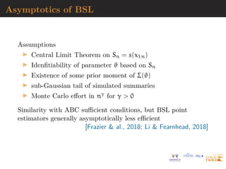
![Asymptotics of BSL
Assumptions
I Central Limit Theorem on Sn = s(x1:n)
I Idenfitiability of parameter ϑ based on Sn
I Existence of some prior moment of Σ(ϑ)
I sub-Gaussian tail of simulated summaries
I Monte Carlo effort in nγ for γ 0
Similarity with ABC sufficient conditions, but BSL point
estimators generally asymptotically less efficient
[Frazier al., 2018; Li Fearnhead, 2018]](https://image.slidesharecdn.com/masterkl-220506133627-ac0e2786/85/CDT-22-slides-pdf-217-320.jpg)
![Asymptotics of ABC
For a sample y = y(n) and a tolerance ε = εn, when n → +∞,
assuming a parametric model ϑ ∈ Rk, k fixed
I Concentration of summary η(z): there exists b(ϑ) such
that
η(z) − b(ϑ) = oPϑ
(1)
I Consistency:
Πεn (kϑ − ϑ0k ≤ δ|y) = 1 + op(1)
I Convergence rate: there exists δn = o(1) such that
Πεn (kϑ − ϑ0k ≤ δn|y) = 1 + op(1)
[Frazier al., 2018]](https://image.slidesharecdn.com/masterkl-220506133627-ac0e2786/85/CDT-22-slides-pdf-218-320.jpg)
![Asymptotics of ABC
Under assumptions
(A1) ∃σn → +∞
Pϑ
σ−1
n kη(z) − b(ϑ)k u
≤ c(ϑ)h(u), lim
u→+∞
h(u) = 0
(A2)
Π(kb(ϑ) − b(ϑ0)k ≤ u) uD
, u ≈ 0
posterior consistency and posterior concentration rate λT that
depends on the deviation control of d2{η(z), b(ϑ)}
posterior concentration rate for b(ϑ) bounded from below by
O(εT )
[Frazier al., 2018]](https://image.slidesharecdn.com/masterkl-220506133627-ac0e2786/85/CDT-22-slides-pdf-219-320.jpg)
![Asymptotics of ABC
Under assumptions
(A1) ∃σn → +∞
Pϑ
σ−1
n kη(z) − b(ϑ)k u
≤ c(ϑ)h(u), lim
u→+∞
h(u) = 0
(A2)
Π(kb(ϑ) − b(ϑ0)k ≤ u) uD
, u ≈ 0
then
Πεn
kb(ϑ) − b(ϑ0)k . εn + σnh−1
(εD
n )|y
= 1 + op0
(1)
If also kϑ − ϑ0k ≤ Lkb(ϑ) − c(ϑ0)kα, locally and ϑ → b(ϑ) 1-1
Πεn (kϑ − ϑ0k . εα
n + σα
n(h−1
(εD
n ))α
| {z }
δn
|y) = 1 + op0
(1)
[Frazier al., 2018]](https://image.slidesharecdn.com/masterkl-220506133627-ac0e2786/85/CDT-22-slides-pdf-220-320.jpg)
![Further ABC assumptions
I (B1) Concentration of summary η: Σn(ϑ) ∈ Rk1×k1 is o(1)
Σn(ϑ)−1
{η(z)−b(ϑ)} ⇒ Nk1
(0, Id), (Σn(ϑ)Σn(ϑ0)−1
)n = Co
I (B2) b(ϑ) is C1 and
kϑ − ϑ0k . kb(ϑ) − b(ϑ0)k
I (B3) Dominated convergence and
lim
n
Pϑ(Σn(ϑ)−1{η(z) − b(ϑ)} ∈ u + B(0, un))
Q
j un(j)
→ ϕ(u)
[Frazier al., 2018]](https://image.slidesharecdn.com/masterkl-220506133627-ac0e2786/85/CDT-22-slides-pdf-221-320.jpg)
![ABC asymptotic regime
Set Σn(ϑ) = σnD(ϑ) for ϑ ≈ ϑ0 and Zo = Σn(ϑ0)−1(η(y) − ϑ0),
then under (B1) and (B2)
I when εnσ−1
n → +∞
Πεn [ε−1
n (ϑ − ϑ0) ∈ A|y] ⇒ UB0 (A), B0 = {x ∈ Rk
; kb0
(ϑ0)T
xk ≤ 1}
I when εnσ−1
n → c
Πεn [Σn(ϑ0)−1
(ϑ − ϑ0) − Zo
∈ A|y] ⇒ Qc(A), Qc 6= N
I when εnσ−1
n → 0 and (B3) holds, set
Vn = [b0
(ϑ0)]T
Σn(ϑ0)b0
(ϑ0)
then
Πεn [V−1
n (ϑ − ϑ0) − Z̃o
∈ A|y] ⇒ Φ(A),
[Frazier al., 2018]](https://image.slidesharecdn.com/masterkl-220506133627-ac0e2786/85/CDT-22-slides-pdf-222-320.jpg)
![conclusion on ABC consistency
I asymptotic description of ABC: different regimes
depending on εn σn
I no point in choosing εn arbitrarily small: just εn = o(σn)
I no gain in iterative ABC
I results under weak conditions by not studying g(η(z)|ϑ)
[Frazier al., 2018]](https://image.slidesharecdn.com/masterkl-220506133627-ac0e2786/85/CDT-22-slides-pdf-223-320.jpg)

This document summarizes techniques for approximating marginal likelihoods and Bayes factors, which are important quantities in Bayesian inference. It discusses Geyer's 1994 logistic regression approach, links to bridge sampling, and how mixtures can be used as importance sampling proposals. Specifically, it shows how optimizing the logistic pseudo-likelihood relates to the bridge sampling optimal estimator. It also discusses non-parametric maximum likelihood estimation based on simulations.


![Human Reproduction [ Reproductive System ] Notes @irfanullah_mehar Irfanullah...](https://cdn.slidesharecdn.com/ss_thumbnails/humanreproductionreproductivesystemnotesirfanullahmeharirfanullahmeharjanantantra-260111172350-56e85778-thumbnail.jpg?width=640&height=640&fit=bounds)
