Download as PDF, PPTX
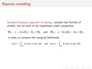
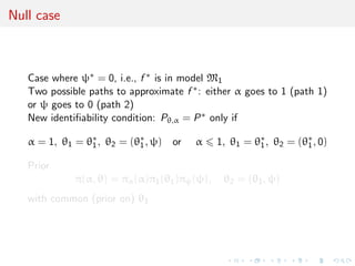
![Introduction
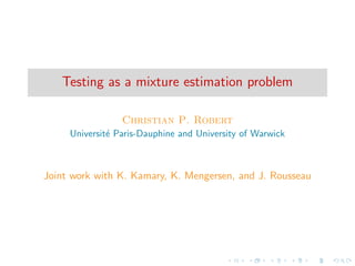
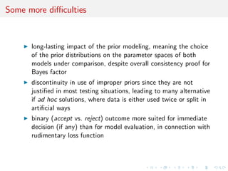
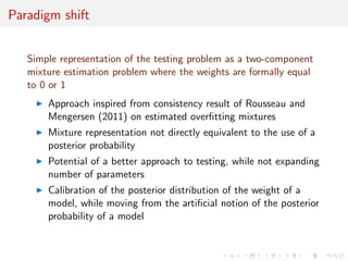
Hypothesis testing
central problem of statistical inference
dramatically differentiating feature between classical and
Bayesian paradigms
wide open to controversy and divergent opinions, even within
the Bayesian community
non-informative Bayesian testing case mostly unresolved,
witness the Jeffreys–Lindley paradox
[Berger (2003), Mayo & Cox (2006), Gelman (2008)]](https://image.slidesharecdn.com/nice-150217005217-conversion-gate02/85/testing-as-a-mixture-estimation-problem-3-320.jpg)

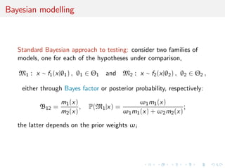

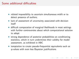
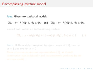
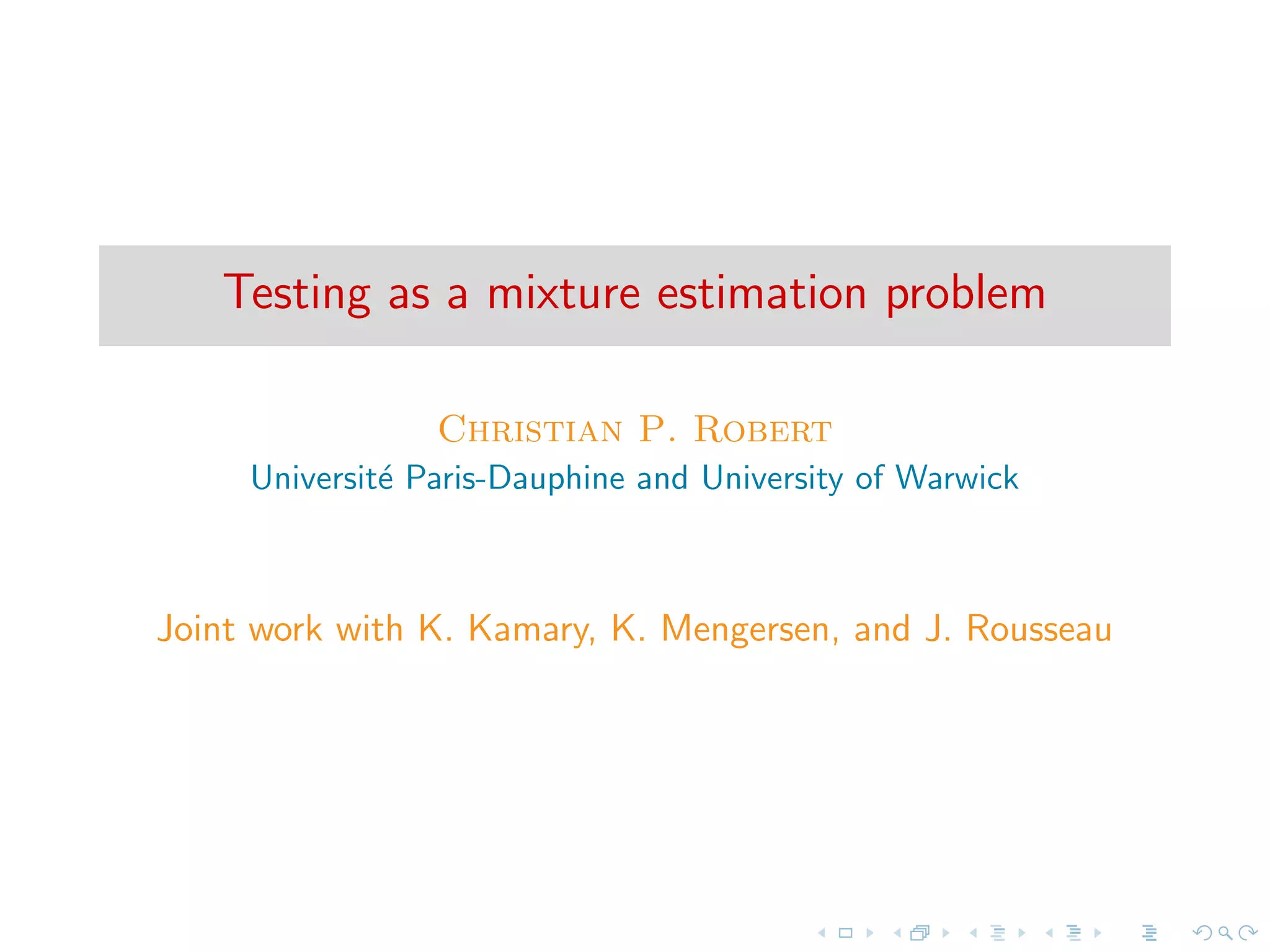
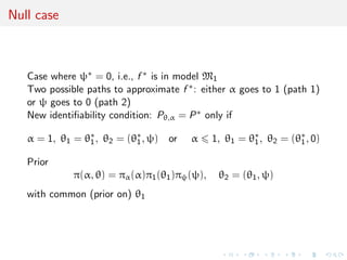
![Gibbs sampler
Consider sample x = (x1, x2, . . . , xn) from (1).
Completion by latent component indicators ζi leads to completed
likelihood
(θ, α1, α2 | x, ζ) =
n
i=1
αζi
f (xi | θζi
)
= αn1
(1 − α)n2
n
i=1
f (xi | θζi
) ,
where
(n1, n2) =
n
i=1
Iζi =1,
n
i=1
Iζi =2
under constraint
n =
2
j=1
n
i=1
Iζi =j
.
[Diebolt & Robert, 1990]](https://image.slidesharecdn.com/nice-150217005217-conversion-gate02/85/testing-as-a-mixture-estimation-problem-24-320.jpg)
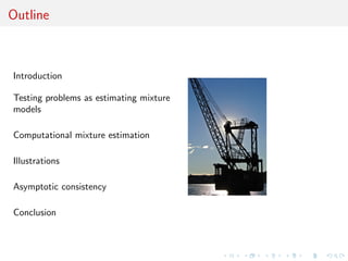
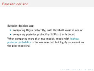
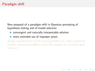
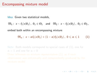
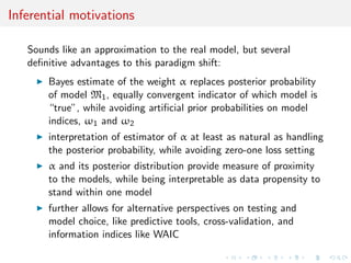
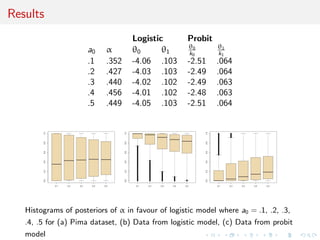
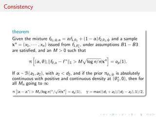
![Comparison with posterior probability
0 100 200 300 400 500
-50-40-30-20-100
a0=.1
sample size
0 100 200 300 400 500
-50-40-30-20-100
a0=.3
sample size
0 100 200 300 400 500
-50-40-30-20-100
a0=.4
sample size
0 100 200 300 400 500
-50-40-30-20-100
a0=.5
sample size
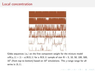
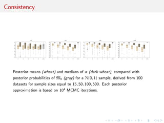
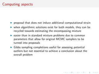
Plots of ranges of log(n) log(1 − E[α|x]) (gray color) and log(1 − p(M1|x)) (red
dotted) over 100 N(0, 1) samples as sample size n grows from 1 to 500. and α
is the weight of N(0, 1) in the mixture model. The shaded areas indicate the
range of the estimations and each plot is based on a Beta prior with
a0 = .1, .2, .3, .4, .5, 1 and each posterior approximation is based on 104
iterations.](https://image.slidesharecdn.com/nice-150217005217-conversion-gate02/85/testing-as-a-mixture-estimation-problem-43-320.jpg)
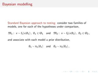
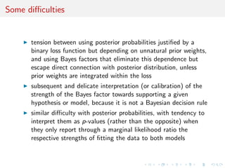
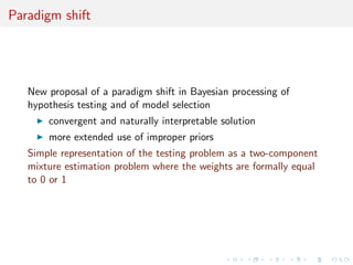
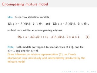
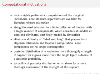
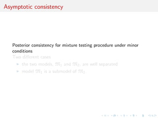
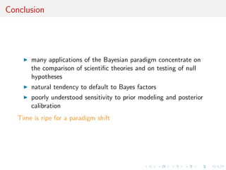
![Common parameterisation
Local reparameterisation strategy that rescales parameters of the
probit model M2 so that the MLE’s of both models coincide.
[Choudhuty et al., 2007]
Φ(xi
θ2) ≈
exp(kxi θ2)
1 + exp(kxi θ2)
and use best estimate of k to bring both parameters into coherency
(k0, k1) = (θ01/θ02, θ11/θ12) ,
reparameterise M1 and M2 as
M1 :yi | xi
, θ ∼ B(1, pi ) where pi =
exp(xi θ)
1 + exp(xi θ)
M2 :yi | xi
, θ ∼ B(1, qi ) where qi = Φ(xi
(κ−1
θ)) ,
with κ−1θ = (θ0/k0, θ1/k1).](https://image.slidesharecdn.com/nice-150217005217-conversion-gate02/85/testing-as-a-mixture-estimation-problem-49-320.jpg)
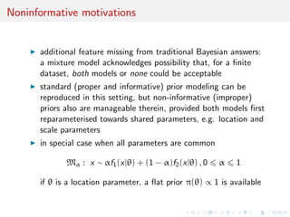
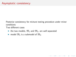
![Prior modelling
Under default g-prior
θ ∼ N2(0, n(XT
X)−1
)
full conditional posterior distributions given allocations
π(θ | y, X, ζ) ∝
exp i Iζi =1yi xi θ
i;ζi =1[1 + exp(xi θ)]
exp −θT
(XT
X)θ 2n
×
i;ζi =2
Φ(xi
(κ−1
θ))yi
(1 − Φ(xi
(κ−1
θ)))(1−yi )
hence posterior distribution clearly defined](https://image.slidesharecdn.com/nice-150217005217-conversion-gate02/85/testing-as-a-mixture-estimation-problem-50-320.jpg)
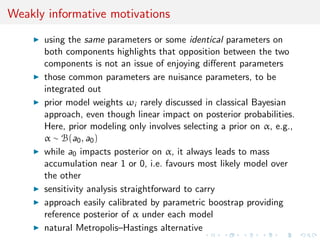
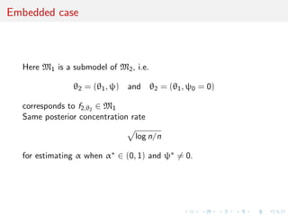
![Posterior concentration rate
Let π be the prior and xn = (x1, · · · , xn) a sample with true
density f ∗
proposition
Assume that, for all c > 0, there exist Θn ⊂ Θ1 × Θ2 and B > 0 such that
π [Θc
n] n−c
, Θn ⊂ { θ1 + θ2 nB
}
and that there exist H 0 and L, δ > 0 such that, for j = 1, 2,
sup
θ,θ ∈Θn
fj,θj
− fj,θj
1 LnH
θj − θj , θ = (θ1, θ2), θ = (θ1, θ2) ,
∀ θj − θ∗
j δ; KL(fj,θj
, fj,θ∗
j
) θj − θ∗
j .
Then, when f ∗
= fθ∗,α∗ , with α∗
∈ [0, 1], there exists M > 0 such that
π (α, θ); fθ,α − f ∗
1 > M log n/n|xn
= op(1) .](https://image.slidesharecdn.com/nice-150217005217-conversion-gate02/85/testing-as-a-mixture-estimation-problem-54-320.jpg)
![Separated models
Assumption: Models are separated, i.e. there is identifiability:
∀α, α ∈ [0, 1], ∀θj , θj , j = 1, 2 Pθ,α = Pθ ,α ⇒ α = α , θ = θ
Further
inf
θ1∈Θ1
inf
θ2∈Θ2
f1,θ1
− f2,θ2 1 > 0
and, for θ∗
j ∈ Θj , if Pθj
weakly converges to Pθ∗
j
, then θj converges
in the Euclidean topology to θ∗
j](https://image.slidesharecdn.com/nice-150217005217-conversion-gate02/85/testing-as-a-mixture-estimation-problem-55-320.jpg)
![Separated models
Assumption: Models are separated, i.e. there is identifiability:
∀α, α ∈ [0, 1], ∀θj , θj , j = 1, 2 Pθ,α = Pθ ,α ⇒ α = α , θ = θ
theorem
Under above assumptions, then for all > 0,
π [|α − α∗
| > |xn
] = op(1)
If θj → fj,θj
is C2 in a neighbourhood of θ∗
j , j = 1, 2,
f1,θ∗
1
− f2,θ∗
2
, f1,θ∗
1
, f2,θ∗
2
are linearly independent in y and there
exists δ > 0 such that
f1,θ∗
1
, f2,θ∗
2
, sup
|θ1−θ∗
1 |<δ
|D2
f1,θ1
|, sup
|θ2−θ∗
2 |<δ
|D2
f2,θ2
| ∈ L1
then
π |α − α∗
| > M log n/n xn
= op(1).](https://image.slidesharecdn.com/nice-150217005217-conversion-gate02/85/testing-as-a-mixture-estimation-problem-56-320.jpg)
![Separated models
Assumption: Models are separated, i.e. there is identifiability:
∀α, α ∈ [0, 1], ∀θj , θj , j = 1, 2 Pθ,α = Pθ ,α ⇒ α = α , θ = θ
Theorem allows for interpretation of α under the posterior: If data
xn is generated from model M1 then posterior on α concentrates
around α = 1](https://image.slidesharecdn.com/nice-150217005217-conversion-gate02/85/testing-as-a-mixture-estimation-problem-57-320.jpg)
![Assumptions
[B1] Regularity: Assume that θ1 → f1,θ1 and θ2 → f2,θ2 are 3
times continuously differentiable and that
F∗
¯f 3
1,θ∗
1
f 3
1,θ∗
1
< +∞, ¯f1,θ∗
1
= sup
|θ1−θ∗
1 |<δ
f1,θ1
, f 1,θ∗
1
= inf
|θ1−θ∗
1 |<δ
f1,θ1
F∗
sup|θ1−θ∗
1 |<δ | f1,θ∗
1
|3
f 3
1,θ∗
1
< +∞, F∗
| f1,θ∗
1
|4
f 4
1,θ∗
1
< +∞,
F∗
sup|θ1−θ∗
1 |<δ |D2
f1,θ∗
1
|2
f 2
1,θ∗
1
< +∞, F∗
sup|θ1−θ∗
1 |<δ |D3
f1,θ∗
1
|
f 1,θ∗
1
< +∞](https://image.slidesharecdn.com/nice-150217005217-conversion-gate02/85/testing-as-a-mixture-estimation-problem-61-320.jpg)
![Assumptions
[B2] Integrability: There exists S0 ⊂ S ∩ {|ψ| > δ0}, for some
positive δ0 and satisfying Leb(S0) > 0, and such that for all
ψ ∈ S0,
F∗
sup|θ1−θ∗
1 |<δ f2,θ1,ψ
f 4
1,θ∗
1
< +∞, F∗
sup|θ1−θ∗
1 |<δ f 3
2,θ1,ψ
f 3
1,θ1∗
< +∞,](https://image.slidesharecdn.com/nice-150217005217-conversion-gate02/85/testing-as-a-mixture-estimation-problem-62-320.jpg)
![Assumptions
[B3] Stronger identifiability : Set
f2,θ∗
1,ψ∗ (x) = θ1 f2,θ∗
1,ψ∗ (x)T
, ψf2,θ∗
1,ψ∗ (x)T T
.
Then for all ψ ∈ S with ψ = 0, if η0 ∈ R, η1 ∈ Rd1
η0(f1,θ∗
1
− f2,θ∗
1,ψ) + ηT
1 θ1 f1,θ∗
1
= 0 ⇔ η1 = 0, η2 = 0](https://image.slidesharecdn.com/nice-150217005217-conversion-gate02/85/testing-as-a-mixture-estimation-problem-63-320.jpg)

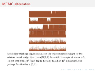
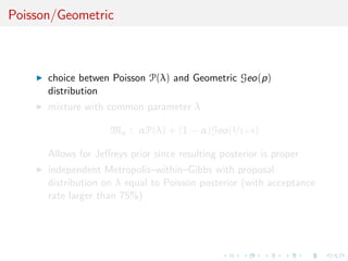
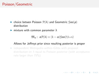
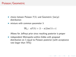
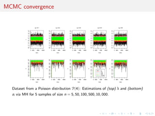
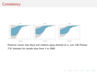
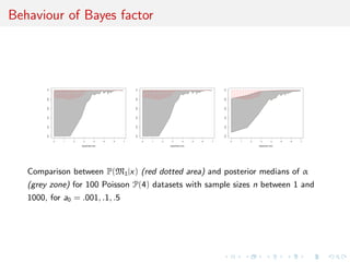
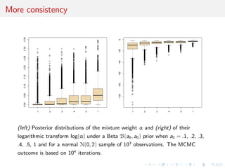
This document proposes representing hypothesis testing problems as estimating mixture models. Specifically, two competing models are embedded within an encompassing mixture model with a weight parameter between 0 and 1. Inference is then drawn on the mixture representation, treating each observation as coming from the mixture model. This avoids difficulties with traditional Bayesian testing approaches like computing marginal likelihoods. It also allows for a more intuitive interpretation of the weight parameter compared to posterior model probabilities. The weight parameter can be estimated using standard mixture estimation algorithms like Gibbs sampling or Metropolis-Hastings. Several illustrations of the approach are provided, including comparisons of Poisson and geometric distributions.


![Polymer [ बहुलक ] Chemistry Notes PDF - Irfanullah Mehar - JJ Sir Chemistry.pdf](https://cdn.slidesharecdn.com/ss_thumbnails/polymerchemistrynotespdf-irfanullahmehar-jjsirchemistry-260210172118-3f9b37f7-thumbnail.jpg?width=640&height=640&fit=bounds)