The document discusses approximate Bayesian computation (ABC), a simulation-based method for conducting Bayesian inference when the likelihood function is intractable or impossible to compute directly. ABC works by simulating data under different parameter values, and accepting simulations that are close to the observed data according to some distance measure. The document covers the basic ABC algorithm, convergence properties as the tolerance approaches zero, examples of ABC for probit models and MA time series models, and advances such as modifying the proposal distribution to increase efficiency.

1. Approximate Bayesian computation
1 simulation-based methods in
Econometrics
2 Genetics of ABC
3 Approximate Bayesian computation
ABC basics
Alphabet soup
ABC as an inference machine
Automated summary statistic
selection
Series B discussion
4 ABC for model choice
5 ABC model choice via random forests

2. Untractable likelihoods
Cases when the likelihood function
f (y|θ) is unavailable and when the
completion step
f (y|θ) =
Z
f (y, z|θ) dz
is impossible or too costly because of
the dimension of z
c MCMC cannot be implemented!

3. Untractable likelihoods
Cases when the likelihood function
f (y|θ) is unavailable and when the
completion step
f (y|θ) =
Z
f (y, z|θ) dz
is impossible or too costly because of
the dimension of z
c MCMC cannot be implemented!

4. Illustration
Example (Ising & Potts models)
Potts model: if y takes values on a grid Y of size kn and
f (y|θ) ∝ exp θ
l∼i
Iyl =yi
where l∼i denotes a neighbourhood relation, n moderately large
prohibits the computation of the normalising constant Zθ

5. Illustration
Example (Ising & Potts models)
Potts model: if y takes values on a grid Y of size kn and
f (y|θ) ∝ exp θ
l∼i
Iyl =yi
where l∼i denotes a neighbourhood relation, n moderately large
prohibits the computation of the normalising constant Zθ
Special case of the intractable normalising constant, making the
likelihood impossible to compute

6. The ABC method
Bayesian setting: target is π(θ)f (x|θ)

7. The ABC method
Bayesian setting: target is π(θ)f (x|θ)
When likelihood f (x|θ) not in closed form, likelihood-free rejection
technique:

8. The ABC method
Bayesian setting: target is π(θ)f (x|θ)
When likelihood f (x|θ) not in closed form, likelihood-free rejection
technique:
ABC algorithm
For an observation y ∼ f (y|θ), under the prior π(θ), keep jointly
simulating
θ ∼ π(θ) , z ∼ f (z|θ ) ,
until the auxiliary variable z is equal to the observed value, z = y.
[Tavar´e et al., 1997]

9. Why does it work?!
The proof is trivial:
f (θi ) ∝
z∈D
π(θi )f (z|θi )Iy(z)
∝ π(θi )f (y|θi )
= π(θi |y) .
[Accept–Reject 101]

10. Earlier occurrence
‘Bayesian statistics and Monte Carlo methods are ideally
suited to the task of passing many models over one
dataset’
[Don Rubin, Annals of Statistics, 1984]
Note Rubin (1984) does not promote this algorithm for
likelihood-free simulation but frequentist intuition on posterior
distributions: parameters from posteriors are more likely to be
those that could have generated the data.

11. A as A...pproximative
When y is a continuous random variable, equality z = y is replaced
with a tolerance condition,
(y, z) ≤
where is a distance

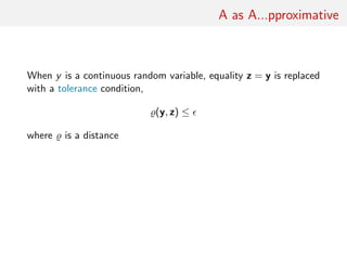
12. A as A...pproximative
When y is a continuous random variable, equality z = y is replaced
with a tolerance condition,
(y, z) ≤
where is a distance
Output distributed from
π(θ) Pθ{ (y, z) < } ∝ π(θ| (y, z) < )
[Pritchard et al., 1999]

13. ABC algorithm
Algorithm 1 Likelihood-free rejection sampler 2
for i = 1 to N do
repeat
generate θ from the prior distribution π(·)
generate z from the likelihood f (·|θ )
until ρ{η(z), η(y)} ≤
set θi = θ
end for
where η(y) defines a (not necessarily sufficient) statistic

14. Output
The likelihood-free algorithm samples from the marginal in z of:
π (θ, z|y) =
π(θ)f (z|θ)IA ,y (z)
A ,y×Θ π(θ)f (z|θ)dzdθ
,
where A ,y = {z ∈ D|ρ(η(z), η(y)) < }.

15. Output
The likelihood-free algorithm samples from the marginal in z of:
π (θ, z|y) =
π(θ)f (z|θ)IA ,y (z)
A ,y×Θ π(θ)f (z|θ)dzdθ
,
where A ,y = {z ∈ D|ρ(η(z), η(y)) < }.
The idea behind ABC is that the summary statistics coupled with a
small tolerance should provide a good approximation of the
posterior distribution:
π (θ|y) = π (θ, z|y)dz ≈ π(θ|y) .

16. Convergence of ABC (first attempt)
What happens when → 0?

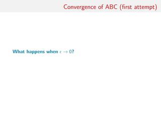
17. Convergence of ABC (first attempt)
What happens when → 0?
If f (·|θ) is continuous in y, uniformly in θ [!], given an arbitrary
δ > 0, there exists 0 such that < 0 implies
π(θ) f (z|θ)IA ,y (z) dz
A ,y×Θ π(θ)f (z|θ)dzdθ
∈
π(θ)f (y|θ)(1 δ)µ(B )
Θ π(θ)f (y|θ)dθ(1 ± δ)µ(B )

18. Convergence of ABC (first attempt)
What happens when → 0?
If f (·|θ) is continuous in y, uniformly in θ [!], given an arbitrary
δ > 0, there exists 0 such that < 0 implies
π(θ) f (z|θ)IA ,y (z) dz
A ,y×Θ π(θ)f (z|θ)dzdθ
∈
π(θ)f (y|θ)(1 δ)XXXXµ(B )
Θ π(θ)f (y|θ)dθ(1 ± δ)XXXXµ(B )

19. Convergence of ABC (first attempt)
What happens when → 0?
If f (·|θ) is continuous in y, uniformly in θ [!], given an arbitrary
δ 0, there exists 0 such that 0 implies
π(θ) f (z|θ)IA ,y (z) dz
A ,y×Θ π(θ)f (z|θ)dzdθ
∈
π(θ)f (y|θ)(1 δ)XXXXµ(B )
Θ π(θ)f (y|θ)dθ(1 ± δ)XXXXµ(B )
[Proof extends to other continuous-in-0 kernels K ]

20. Convergence of ABC (second attempt)
What happens when → 0?

21. Convergence of ABC (second attempt)
What happens when → 0?
For B ⊂ Θ, we have
B
A ,y
f (z|θ)dz
A ,y×Θ π(θ)f (z|θ)dzdθ
π(θ)dθ =
A ,y
B f (z|θ)π(θ)dθ
A ,y×Θ π(θ)f (z|θ)dzdθ
dz
=
A ,y
B f (z|θ)π(θ)dθ
m(z)
m(z)
A ,y×Θ π(θ)f (z|θ)dzdθ
dz
=
A ,y
π(B|z)
m(z)
A ,y×Θ π(θ)f (z|θ)dzdθ
dz
which indicates convergence for a continuous π(B|z).

22. Probit modelling on Pima Indian women
Example (R benchmark)
200 Pima Indian women with observed variables
• plasma glucose concentration in oral glucose tolerance test
• diastolic blood pressure
• diabetes pedigree function
• presence/absence of diabetes

23. Probit modelling on Pima Indian women
Example (R benchmark)
200 Pima Indian women with observed variables
• plasma glucose concentration in oral glucose tolerance test
• diastolic blood pressure
• diabetes pedigree function
• presence/absence of diabetes
Probability of diabetes function of above variables
P(y = 1|x) = Φ(x1β1 + x2β2 + x3β3) ,

24. Probit modelling on Pima Indian women
Example (R benchmark)
200 Pima Indian women with observed variables
• plasma glucose concentration in oral glucose tolerance test
• diastolic blood pressure
• diabetes pedigree function
• presence/absence of diabetes
Probability of diabetes function of above variables
P(y = 1|x) = Φ(x1β1 + x2β2 + x3β3) ,
Test of H0 : β3 = 0 for 200 observations of Pima.tr based on a
g-prior modelling:
β ∼ N3(0, n XT
X)−1

25. Probit modelling on Pima Indian women
Example (R benchmark)
200 Pima Indian women with observed variables
• plasma glucose concentration in oral glucose tolerance test
• diastolic blood pressure
• diabetes pedigree function
• presence/absence of diabetes
Probability of diabetes function of above variables
P(y = 1|x) = Φ(x1β1 + x2β2 + x3β3) ,
Test of H0 : β3 = 0 for 200 observations of Pima.tr based on a
g-prior modelling:
β ∼ N3(0, n XT
X)−1
Use of importance function inspired from the MLE estimate
distribution
β ∼ N(ˆβ, ˆΣ)

26. Pima Indian benchmark
−0.005 0.010 0.020 0.030
020406080100
Density
−0.05 −0.03 −0.01
020406080
Density
−1.0 0.0 1.0 2.0
0.00.20.40.60.81.0
Density
Figure: Comparison between density estimates of the marginals on β1
(left), β2 (center) and β3 (right) from ABC rejection samples (red) and
MCMC samples (black)
.

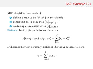
27. MA example
Back to the MA(q) model
xt = t +
q
i=1
ϑi t−i
Simple prior: uniform over the inverse [real and complex] roots in
Q(u) = 1 −
q
i=1
ϑi ui
under the identifiability conditions

28. MA example
Back to the MA(q) model
xt = t +
q
i=1
ϑi t−i
Simple prior: uniform prior over the identifiability zone, e.g.
triangle for MA(2)

29. MA example (2)
ABC algorithm thus made of
1 picking a new value (ϑ1, ϑ2) in the triangle
2 generating an iid sequence ( t)−qt≤T
3 producing a simulated series (xt)1≤t≤T

30. MA example (2)
ABC algorithm thus made of
1 picking a new value (ϑ1, ϑ2) in the triangle
2 generating an iid sequence ( t)−qt≤T
3 producing a simulated series (xt)1≤t≤T
Distance: basic distance between the series
ρ((xt)1≤t≤T , (xt)1≤t≤T ) =
T
t=1
(xt − xt)2
or distance between summary statistics like the q autocorrelations
τj =
T
t=j+1
xtxt−j

31. Comparison of distance impact
Evaluation of the tolerance on the ABC sample against both
distances ( = 100%, 10%, 1%, 0.1%) for an MA(2) model

32. Comparison of distance impact
0.0 0.2 0.4 0.6 0.8
01234
θ1
−2.0 −1.0 0.0 0.5 1.0 1.5
0.00.51.01.5
θ2
Evaluation of the tolerance on the ABC sample against both
distances ( = 100%, 10%, 1%, 0.1%) for an MA(2) model

33. Comparison of distance impact
0.0 0.2 0.4 0.6 0.8
01234
θ1
−2.0 −1.0 0.0 0.5 1.0 1.5
0.00.51.01.5
θ2
Evaluation of the tolerance on the ABC sample against both
distances ( = 100%, 10%, 1%, 0.1%) for an MA(2) model

34. Homonomy
The ABC algorithm is not to be confused with the ABC algorithm
The Artificial Bee Colony algorithm is a swarm based meta-heuristic
algorithm that was introduced by Karaboga in 2005 for optimizing
numerical problems. It was inspired by the intelligent foraging
behavior of honey bees. The algorithm is specifically based on the
model proposed by Tereshko and Loengarov (2005) for the foraging
behaviour of honey bee colonies. The model consists of three
essential components: employed and unemployed foraging bees, and
food sources. The first two components, employed and unemployed
foraging bees, search for rich food sources (...) close to their hive.
The model also defines two leading modes of behaviour (...):
recruitment of foragers to rich food sources resulting in positive
feedback and abandonment of poor sources by foragers causing
negative feedback.
[Karaboga, Scholarpedia]

35. ABC advances
Simulating from the prior is often poor in efficiency

36. ABC advances
Simulating from the prior is often poor in efficiency
Either modify the proposal distribution on θ to increase the density
of x’s within the vicinity of y...
[Marjoram et al, 2003; Bortot et al., 2007, Sisson et al., 2007]

37. ABC advances
Simulating from the prior is often poor in efficiency
Either modify the proposal distribution on θ to increase the density
of x’s within the vicinity of y...
[Marjoram et al, 2003; Bortot et al., 2007, Sisson et al., 2007]
...or by viewing the problem as a conditional density estimation
and by developing techniques to allow for larger
[Beaumont et al., 2002]

38. ABC advances
Simulating from the prior is often poor in efficiency
Either modify the proposal distribution on θ to increase the density
of x’s within the vicinity of y...
[Marjoram et al, 2003; Bortot et al., 2007, Sisson et al., 2007]
...or by viewing the problem as a conditional density estimation
and by developing techniques to allow for larger
[Beaumont et al., 2002]
.....or even by including in the inferential framework [ABCµ]
[Ratmann et al., 2009]

39. ABC-NP
Better usage of [prior] simulations by
adjustement: instead of throwing away
θ such that ρ(η(z), η(y)) , replace
θ’s with locally regressed transforms
(use with BIC)
θ∗
= θ − {η(z) − η(y)}T ˆβ [Csill´ery et al., TEE, 2010]
where ˆβ is obtained by [NP] weighted least square regression on
(η(z) − η(y)) with weights
Kδ {ρ(η(z), η(y))}
[Beaumont et al., 2002, Genetics]

40. ABC-NP (regression)
Also found in the subsequent literature, e.g. in Fearnhead-Prangle (2012) :
weight directly simulation by
Kδ {ρ(η(z(θ)), η(y))}
or
1
S
S
s=1
Kδ {ρ(η(zs
(θ)), η(y))}
[consistent estimate of f (η|θ)]

41. ABC-NP (regression)
Also found in the subsequent literature, e.g. in Fearnhead-Prangle (2012) :
weight directly simulation by
Kδ {ρ(η(z(θ)), η(y))}
or
1
S
S
s=1
Kδ {ρ(η(zs
(θ)), η(y))}
[consistent estimate of f (η|θ)]
Curse of dimensionality: poor estimate when d = dim(η) is large...

42. ABC-NP (density estimation)
Use of the kernel weights
Kδ {ρ(η(z(θ)), η(y))}
leads to the NP estimate of the posterior expectation
i θi Kδ {ρ(η(z(θi )), η(y))}
i Kδ {ρ(η(z(θi )), η(y))}
[Blum, JASA, 2010]

43. ABC-NP (density estimation)
Use of the kernel weights
Kδ {ρ(η(z(θ)), η(y))}
leads to the NP estimate of the posterior conditional density
i
˜Kb(θi − θ)Kδ {ρ(η(z(θi )), η(y))}
i Kδ {ρ(η(z(θi )), η(y))}
[Blum, JASA, 2010]

44. ABC-NP (density estimations)
Other versions incorporating regression adjustments
i
˜Kb(θ∗
i − θ)Kδ {ρ(η(z(θi )), η(y))}
i Kδ {ρ(η(z(θi )), η(y))}

45. ABC-NP (density estimations)
Other versions incorporating regression adjustments
i
˜Kb(θ∗
i − θ)Kδ {ρ(η(z(θi )), η(y))}
i Kδ {ρ(η(z(θi )), η(y))}
In all cases, error
E[ˆg(θ|y)] − g(θ|y) = cb2
+ cδ2
+ OP(b2
+ δ2
) + OP(1/nδd
)
var(ˆg(θ|y)) =
c
nbδd
(1 + oP(1))
[Blum, JASA, 2010]

46. ABC-NP (density estimations)
Other versions incorporating regression adjustments
i
˜Kb(θ∗
i − θ)Kδ {ρ(η(z(θi )), η(y))}
i Kδ {ρ(η(z(θi )), η(y))}
In all cases, error
E[ˆg(θ|y)] − g(θ|y) = cb2
+ cδ2
+ OP(b2
+ δ2
) + OP(1/nδd
)
var(ˆg(θ|y)) =
c
nbδd
(1 + oP(1))
[standard NP calculations]

47. ABC-NCH
Incorporating non-linearities and heterocedasticities:
θ∗
= ˆm(η(y)) + [θ − ˆm(η(z))]
ˆσ(η(y))
ˆσ(η(z))

48. ABC-NCH
Incorporating non-linearities and heterocedasticities:
θ∗
= ˆm(η(y)) + [θ − ˆm(η(z))]
ˆσ(η(y))
ˆσ(η(z))
where
• ˆm(η) estimated by non-linear regression (e.g., neural network)
• ˆσ(η) estimated by non-linear regression on residuals
log{θi − ˆm(ηi )}2
= log σ2
(ηi ) + ξi
[Blum Fran¸cois, 2009]

49. ABC-NCH (2)
Why neural network?

50. ABC-NCH (2)
Why neural network?
• fights curse of dimensionality
• selects relevant summary statistics
• provides automated dimension reduction
• offers a model choice capability
• improves upon multinomial logistic
[Blum Fran¸cois, 2009]

51. ABC as knn
[Biau et al., 2013, Annales de l’IHP]
Practice of ABC: determine tolerance as a quantile on observed
distances, say 10% or 1% quantile,
= N = qα(d1, . . . , dN)

52. ABC as knn
[Biau et al., 2013, Annales de l’IHP]
Practice of ABC: determine tolerance as a quantile on observed
distances, say 10% or 1% quantile,
= N = qα(d1, . . . , dN)
• Interpretation of ε as nonparametric bandwidth only
approximation of the actual practice
[Blum Fran¸cois, 2010]

53. ABC as knn
[Biau et al., 2013, Annales de l’IHP]
Practice of ABC: determine tolerance as a quantile on observed
distances, say 10% or 1% quantile,
= N = qα(d1, . . . , dN)
• Interpretation of ε as nonparametric bandwidth only
approximation of the actual practice
[Blum Fran¸cois, 2010]
• ABC is a k-nearest neighbour (knn) method with kN = N N
[Loftsgaarden Quesenberry, 1965]

54. ABC consistency
Provided
kN/ log log N −→ ∞ and kN/N −→ 0
as N → ∞, for almost all s0 (with respect to the distribution of
S), with probability 1,
1
kN
kN
j=1
ϕ(θj ) −→ E[ϕ(θj )|S = s0]
[Devroye, 1982]

55. ABC consistency
Provided
kN/ log log N −→ ∞ and kN/N −→ 0
as N → ∞, for almost all s0 (with respect to the distribution of
S), with probability 1,
1
kN
kN
j=1
ϕ(θj ) −→ E[ϕ(θj )|S = s0]
[Devroye, 1982]
Biau et al. (2013) also recall pointwise and integrated mean square error
consistency results on the corresponding kernel estimate of the
conditional posterior distribution, under constraints
kN → ∞, kN /N → 0, hN → 0 and hp
N kN → ∞,

56. Rates of convergence
Further assumptions (on target and kernel) allow for precise
(integrated mean square) convergence rates (as a power of the
sample size N), derived from classical k-nearest neighbour
regression, like
• when m = 1, 2, 3, kN ≈ N(p+4)/(p+8) and rate N
− 4
p+8
• when m = 4, kN ≈ N(p+4)/(p+8) and rate N
− 4
p+8 log N
• when m 4, kN ≈ N(p+4)/(m+p+4) and rate N
− 4
m+p+4
[Biau et al., 2013]

57. Rates of convergence
Further assumptions (on target and kernel) allow for precise
(integrated mean square) convergence rates (as a power of the
sample size N), derived from classical k-nearest neighbour
regression, like
• when m = 1, 2, 3, kN ≈ N(p+4)/(p+8) and rate N
− 4
p+8
• when m = 4, kN ≈ N(p+4)/(p+8) and rate N
− 4
p+8 log N
• when m 4, kN ≈ N(p+4)/(m+p+4) and rate N
− 4
m+p+4
[Biau et al., 2013]
Drag: Only applies to sufficient summary statistics

58. How Bayesian is aBc..?
• may be a convergent method of inference (meaningful?
sufficient? foreign?)
• approximation error unknown (w/o massive simulation)
• pragmatic/empirical B (there is no other solution!)
• many calibration issues (tolerance, distance, statistics)
• the NP side should be incorporated into the whole B picture
• the approximation error should also be part of the B inference

59. ABC-MCMC
Markov chain (θ(t)) created via the transition function
θ(t+1)
=



θ ∼ Kω(θ |θ(t)) if x ∼ f (x|θ ) is such that x = y
and u ∼ U(0, 1) ≤ π(θ )Kω(θ(t)|θ )
π(θ(t))Kω(θ |θ(t))
,
θ(t) otherwise,

60. ABC-MCMC
Markov chain (θ(t)) created via the transition function
θ(t+1)
=



θ ∼ Kω(θ |θ(t)) if x ∼ f (x|θ ) is such that x = y
and u ∼ U(0, 1) ≤ π(θ )Kω(θ(t)|θ )
π(θ(t))Kω(θ |θ(t))
,
θ(t) otherwise,
has the posterior π(θ|y) as stationary distribution
[Marjoram et al, 2003]

61. ABC-MCMC (2)
Algorithm 2 Likelihood-free MCMC sampler
Use Algorithm 1 to get (θ(0), z(0))
for t = 1 to N do
Generate θ from Kω ·|θ(t−1) ,
Generate z from the likelihood f (·|θ ),
Generate u from U[0,1],
if u ≤ π(θ )Kω(θ(t−1)|θ )
π(θ(t−1)Kω(θ |θ(t−1))
IA ,y (z ) then
set (θ(t), z(t)) = (θ , z )
else
(θ(t), z(t))) = (θ(t−1), z(t−1)),
end if
end for

62. Why does it work?
Acceptance probability does not involve calculating the likelihood
and
π (θ , z |y)
π (θ(t−1)
, z(t−1)|y)
×
q(θ(t−1)
|θ )f (z(t−1)|θ(t−1)
)
q(θ |θ(t−1)
)f (z |θ )
=
π(θ ) XXXXf (z |θ ) IA ,y (z )
π(θ(t−1)
) f (z(t−1)|θ(t−1)
) IA ,y (z(t−1))
×
q(θ(t−1)
|θ ) f (z(t−1)|θ(t−1)
)
q(θ |θ(t−1)
) XXXXf (z |θ )

63. Why does it work?
Acceptance probability does not involve calculating the likelihood
and
π (θ , z |y)
π (θ(t−1)
, z(t−1)|y)
×
q(θ(t−1)
|θ )f (z(t−1)|θ(t−1)
)
q(θ |θ(t−1)
)f (z |θ )
=
π(θ ) XXXXf (z |θ ) IA ,y (z )
π(θ(t−1)
)((((((((hhhhhhhhf (z(t−1)|θ(t−1)
) IA ,y (z(t−1))
×
q(θ(t−1)
|θ ) ((((((((hhhhhhhhf (z(t−1)|θ(t−1)
)
q(θ |θ(t−1)
) XXXXf (z |θ )

64. Why does it work?
Acceptance probability does not involve calculating the likelihood
and
π (θ , z |y)
π (θ(t−1)
, z(t−1)|y)
×
q(θ(t−1)
|θ )f (z(t−1)|θ(t−1)
)
q(θ |θ(t−1)
)f (z |θ )
=
π(θ ) XXXXf (z |θ ) IA ,y (z )
π(θ(t−1)
)((((((((hhhhhhhhf (z(t−1)|θ(t−1)
)XXXXXXIA ,y (z(t−1))
×
q(θ(t−1)
|θ ) ((((((((hhhhhhhhf (z(t−1)|θ(t−1)
)
q(θ |θ(t−1)
) XXXXf (z |θ )
=
π(θ )q(θ(t−1)
|θ )
π(θ(t−1)
q(θ |θ(t−1)
)
IA ,y (z )

65. ABCµ
[Ratmann, Andrieu, Wiuf and Richardson, 2009, PNAS]
Use of a joint density
f (θ, |y) ∝ ξ( |y, θ) × πθ(θ) × π ( )
where y is the data, and ξ( |y, θ) is the prior predictive density of
ρ(η(z), η(y)) given θ and y when z ∼ f (z|θ)

66. ABCµ
[Ratmann, Andrieu, Wiuf and Richardson, 2009, PNAS]
Use of a joint density
f (θ, |y) ∝ ξ( |y, θ) × πθ(θ) × π ( )
where y is the data, and ξ( |y, θ) is the prior predictive density of
ρ(η(z), η(y)) given θ and y when z ∼ f (z|θ)
Warning! Replacement of ξ( |y, θ) with a non-parametric kernel
approximation.

67. ABCµ details
Multidimensional distances ρk (k = 1, . . . , K) and errors
k = ρk(ηk(z), ηk(y)), with
k ∼ ξk( |y, θ) ≈ ˆξk( |y, θ) =
1
Bhk
b
K[{ k−ρk(ηk(zb), ηk(y))}/hk]
then used in replacing ξ( |y, θ) with mink
ˆξk( |y, θ)

68. ABCµ details
Multidimensional distances ρk (k = 1, . . . , K) and errors
k = ρk(ηk(z), ηk(y)), with
k ∼ ξk( |y, θ) ≈ ˆξk( |y, θ) =
1
Bhk
b
K[{ k−ρk(ηk(zb), ηk(y))}/hk]
then used in replacing ξ( |y, θ) with mink
ˆξk( |y, θ)
ABCµ involves acceptance probability
π(θ , )
π(θ, )
q(θ , θ)q( , )
q(θ, θ )q( , )
mink
ˆξk( |y, θ )
mink
ˆξk( |y, θ)

69. ABCµ multiple errors
[ c Ratmann et al., PNAS, 2009]

70. ABCµ for model choice
[ c Ratmann et al., PNAS, 2009]

71. Questions about ABCµ
For each model under comparison, marginal posterior on used to
assess the fit of the model (HPD includes 0 or not).

72. Questions about ABCµ
For each model under comparison, marginal posterior on used to
assess the fit of the model (HPD includes 0 or not).
• Is the data informative about ? [Identifiability]
• How is the prior π( ) impacting the comparison?
• How is using both ξ( |x0, θ) and π ( ) compatible with a
standard probability model? [remindful of Wilkinson ]
• Where is the penalisation for complexity in the model
comparison?
[X, Mengersen Chen, 2010, PNAS]

73. A PMC version
Use of the same kernel idea as ABC-PRC (Sisson et al., 2007) but
with IS correction
Generate a sample at iteration t by
ˆπt(θ(t)
) ∝
N
j=1
ω
(t−1)
j Kt(θ(t)
|θ
(t−1)
j )
modulo acceptance of the associated xt, and use an importance
weight associated with an accepted simulation θ
(t)
i
ω
(t)
i ∝ π(θ
(t)
i ) ˆπt(θ
(t)
i ) .
c Still likelihood free
[Beaumont et al., 2009]

74. ABC-PMC algorithm
Given a decreasing sequence of approximation levels 1 ≥ . . . ≥ T ,
1. At iteration t = 1,
For i = 1, ..., N
Simulate θ
(1)
i ∼ π(θ) and x ∼ f (x|θ
(1)
i ) until (x, y) 1
Set ω
(1)
i = 1/N
Take τ2
as twice the empirical variance of the θ
(1)
i ’s
2. At iteration 2 ≤ t ≤ T,
For i = 1, ..., N, repeat
Pick θi from the θ
(t−1)
j ’s with probabilities ω
(t−1)
j
generate θ
(t)
i |θi ∼ N(θi , σ2
t ) and x ∼ f (x|θ
(t)
i )
until (x, y) t
Set ω
(t)
i ∝ π(θ
(t)
i )/ N
j=1 ω
(t−1)
j ϕ σ−1
t θ
(t)
i − θ
(t−1)
j )
Take τ2
t+1 as twice the weighted empirical variance of the θ
(t)
i ’s

75. Sequential Monte Carlo
SMC is a simulation technique that approximates a sequence of
related probability distributions πn with π0 “easy” and πT as
target.
Iterated IS as PMC: particles moved from time n to time n via
kernel Kn and use of a sequence of extended targets ˜πn
˜πn(z0:n) = πn(zn)
n
j=0
Lj (zj+1, zj )
where the Lj ’s are backward Markov kernels [check that πn(zn) is a
marginal]
[Del Moral, Doucet Jasra, Series B, 2006]

76. Sequential Monte Carlo (2)
Algorithm 3 SMC sampler
sample z
(0)
i ∼ γ0(x) (i = 1, . . . , N)
compute weights w
(0)
i = π0(z
(0)
i )/γ0(z
(0)
i )
for t = 1 to N do
if ESS(w(t−1)) NT then
resample N particles z(t−1) and set weights to 1
end if
generate z
(t−1)
i ∼ Kt(z
(t−1)
i , ·) and set weights to
w
(t)
i = w
(t−1)
i−1
πt(z
(t)
i ))Lt−1(z
(t)
i ), z
(t−1)
i ))
πt−1(z
(t−1)
i ))Kt(z
(t−1)
i ), z
(t)
i ))
end for
[Del Moral, Doucet Jasra, Series B, 2006]

77. ABC-SMC
[Del Moral, Doucet Jasra, 2009]
True derivation of an SMC-ABC algorithm
Use of a kernel Kn associated with target π n and derivation of the
backward kernel
Ln−1(z, z ) =
π n (z )Kn(z , z)
πn(z)
Update of the weights
win ∝ wi(n−1)
M
m=1 IA n
(xm
in )
M
m=1 IA n−1
(xm
i(n−1))
when xm
in ∼ K(xi(n−1), ·)

78. ABC-SMCM
Modification: Makes M repeated simulations of the pseudo-data z
given the parameter, rather than using a single [M = 1] simulation,
leading to weight that is proportional to the number of accepted
zi s
ω(θ) =
1
M
M
i=1
Iρ(η(y),η(zi ))
[limit in M means exact simulation from (tempered) target]

79. Properties of ABC-SMC
The ABC-SMC method properly uses a backward kernel L(z, z ) to
simplify the importance weight and to remove the dependence on
the unknown likelihood from this weight. Update of importance
weights is reduced to the ratio of the proportions of surviving
particles
Major assumption: the forward kernel K is supposed to be invariant
against the true target [tempered version of the true posterior]

80. Properties of ABC-SMC
The ABC-SMC method properly uses a backward kernel L(z, z ) to
simplify the importance weight and to remove the dependence on
the unknown likelihood from this weight. Update of importance
weights is reduced to the ratio of the proportions of surviving
particles
Major assumption: the forward kernel K is supposed to be invariant
against the true target [tempered version of the true posterior]
Adaptivity in ABC-SMC algorithm only found in on-line
construction of the thresholds t, slowly enough to keep a large
number of accepted transitions

81. A mixture example (2)
Recovery of the target, whether using a fixed standard deviation of
τ = 0.15 or τ = 1/0.15, or a sequence of adaptive τt’s.
θθ
−3 −2 −1 0 1 2 3
0.00.20.40.60.81.0
θθ
−3 −2 −1 0 1 2 3
0.00.20.40.60.81.0
θθ
−3 −2 −1 0 1 2 3
0.00.20.40.60.81.0
θθ
−3 −2 −1 0 1 2 3
0.00.20.40.60.81.0
θθ
−3 −2 −1 0 1 2 3
0.00.20.40.60.81.0

82. Wilkinson’s exact BC
ABC approximation error (i.e. non-zero tolerance) replaced with
exact simulation from a controlled approximation to the target,
convolution of true posterior with kernel function
π (θ, z|y) =
π(θ)f (z|θ)K (y − z)
π(θ)f (z|θ)K (y − z)dzdθ
,
with K kernel parameterised by bandwidth .
[Wilkinson, 2008]

83. Wilkinson’s exact BC
ABC approximation error (i.e. non-zero tolerance) replaced with
exact simulation from a controlled approximation to the target,
convolution of true posterior with kernel function
π (θ, z|y) =
π(θ)f (z|θ)K (y − z)
π(θ)f (z|θ)K (y − z)dzdθ
,
with K kernel parameterised by bandwidth .
[Wilkinson, 2008]
Theorem
The ABC algorithm based on the assumption of a randomised
observation y = ˜y + ξ, ξ ∼ K , and an acceptance probability of
K (y − z)/M
gives draws from the posterior distribution π(θ|y).

84. How exact a BC?
“Using to represent measurement error is
straightforward, whereas using to model the model
discrepancy is harder to conceptualize and not as
commonly used”
[Richard Wilkinson, 2008, 2013]

85. How exact a BC?
Pros
• Pseudo-data from true model and observed data from noisy
model
• Interesting perspective in that outcome is completely
controlled
• Link with ABCµ and assuming y is observed with a
measurement error with density K
• Relates to the theory of model approximation
[Kennedy O’Hagan, 2001]
Cons
• Requires K to be bounded by M
• True approximation error never assessed
• Requires a modification of the standard ABC algorithm

86. Noisy ABC
Idea: Modify the data from the start
˜y = y0 + ζ1
with the same scale as ABC
[ see Fearnhead-Prangle ]
run ABC on ˜y

87. Noisy ABC
Idea: Modify the data from the start
˜y = y0 + ζ1
with the same scale as ABC
[ see Fearnhead-Prangle ]
run ABC on ˜y
Then ABC produces an exact simulation from π(θ|˜y) = π(θ|˜y)
[Dean et al., 2011; Fearnhead and Prangle, 2012]

88. Consistent noisy ABC
• Degrading the data improves the estimation performances:
• Noisy ABC-MLE is asymptotically (in n) consistent
• under further assumptions, the noisy ABC-MLE is
asymptotically normal
• increase in variance of order −2
• likely degradation in precision or computing time due to the
lack of summary statistic [curse of dimensionality]

89. Semi-automatic ABC
Fearnhead and Prangle (2010) study ABC and the selection of the
summary statistic in close proximity to Wilkinson’s proposal
ABC then considered from a purely inferential viewpoint and
calibrated for estimation purposes
Use of a randomised (or ‘noisy’) version of the summary statistics
˜η(y) = η(y) + τ
Derivation of a well-calibrated version of ABC, i.e. an algorithm
that gives proper predictions for the distribution associated with
this randomised summary statistic

90. Semi-automatic ABC
Fearnhead and Prangle (2010) study ABC and the selection of the
summary statistic in close proximity to Wilkinson’s proposal
ABC then considered from a purely inferential viewpoint and
calibrated for estimation purposes
Use of a randomised (or ‘noisy’) version of the summary statistics
˜η(y) = η(y) + τ
Derivation of a well-calibrated version of ABC, i.e. an algorithm
that gives proper predictions for the distribution associated with
this randomised summary statistic [calibration constraint: ABC
approximation with same posterior mean as the true randomised
posterior]

91. Summary statistics
• Optimality of the posterior expectation E[θ|y] of the
parameter of interest as summary statistics η(y)!

92. Summary statistics
• Optimality of the posterior expectation E[θ|y] of the
parameter of interest as summary statistics η(y)!
• Use of the standard quadratic loss function
(θ − θ0)T
A(θ − θ0) .
bare summary

93. Details on Fearnhead and Prangle (FP) ABC
Use of a summary statistic S(·), an importance proposal g(·), a
kernel K(·) ≤ 1 and a bandwidth h 0 such that
(θ, ysim) ∼ g(θ)f (ysim|θ)
is accepted with probability (hence the bound)
K[{S(ysim) − sobs}/h]
and the corresponding importance weight defined by
π(θ) g(θ)
[Fearnhead Prangle, 2012]

94. Errors, errors, and errors
Three levels of approximation
• π(θ|yobs) by π(θ|sobs) loss of information
[ignored]
• π(θ|sobs) by
πABC(θ|sobs) =
π(s)K[{s − sobs}/h]π(θ|s) ds
π(s)K[{s − sobs}/h] ds
noisy observations
• πABC(θ|sobs) by importance Monte Carlo based on N
simulations, represented by var(a(θ)|sobs)/Nacc [expected
number of acceptances]
[M. Twain/B. Disraeli]

95. Average acceptance asymptotics
For the average acceptance probability/approximate likelihood
p(θ|sobs) = f (ysim|θ) K[{S(ysim) − sobs}/h] dysim ,
overall acceptance probability
p(sobs) = p(θ|sobs) π(θ) dθ = π(sobs)hd
+ o(hd
)
[FP, Lemma 1]

96. Optimal importance proposal
Best choice of importance proposal in terms of effective sample size
g (θ|sobs) ∝ π(θ)p(θ|sobs)1/2
[Not particularly useful in practice]

97. Optimal importance proposal
Best choice of importance proposal in terms of effective sample size
g (θ|sobs) ∝ π(θ)p(θ|sobs)1/2
[Not particularly useful in practice]
• note that p(θ|sobs) is an approximate likelihood
• reminiscent of parallel tempering
• could be approximately achieved by attrition of half of the
data

98. Calibration of h
“This result gives insight into how S(·) and h affect the Monte
Carlo error. To minimize Monte Carlo error, we need hd
to be not
too small. Thus ideally we want S(·) to be a low dimensional
summary of the data that is sufficiently informative about θ that
π(θ|sobs) is close, in some sense, to π(θ|yobs)” (FP, p.5)
• turns h into an absolute value while it should be
context-dependent and user-calibrated
• only addresses one term in the approximation error and
acceptance probability (“curse of dimensionality”)
• h large prevents πABC(θ|sobs) to be close to π(θ|sobs)
• d small prevents π(θ|sobs) to be close to π(θ|yobs) (“curse of
[dis]information”)

99. Calibrating ABC
“If πABC is calibrated, then this means that probability statements
that are derived from it are appropriate, and in particular that we
can use πABC to quantify uncertainty in estimates” (FP, p.5)

100. Calibrating ABC
“If πABC is calibrated, then this means that probability statements
that are derived from it are appropriate, and in particular that we
can use πABC to quantify uncertainty in estimates” (FP, p.5)
Definition
For 0 q 1 and subset A, event Eq(A) made of sobs such that
PrABC(θ ∈ A|sobs) = q. Then ABC is calibrated if
Pr(θ ∈ A|Eq(A)) = q
• unclear meaning of conditioning on Eq(A)

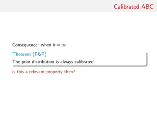
101. Calibrated ABC
Theorem (FP)
Noisy ABC, where
sobs = S(yobs) + h , ∼ K(·)
is calibrated
[Wilkinson, 2008]
no condition on h!!

102. Calibrated ABC
Consequence: when h = ∞
Theorem (FP)
The prior distribution is always calibrated
is this a relevant property then?

103. More about calibrated ABC
“Calibration is not universally accepted by Bayesians. It is even more
questionable here as we care how statements we make relate to the
real world, not to a mathematically defined posterior.” R. Wilkinson
• Same reluctance about the prior being calibrated
• Property depending on prior, likelihood, and summary
• Calibration is a frequentist property (almost a p-value!)
• More sensible to account for the simulator’s imperfections
than using noisy-ABC against a meaningless based measure
[Wilkinson, 2012]

104. Converging ABC
Theorem (FP)
For noisy ABC, the expected noisy-ABC log-likelihood,
E {log[p(θ|sobs)]} = log[p(θ|S(yobs) + )]π(yobs|θ0)K( )dyobsd ,
has its maximum at θ = θ0.
True for any choice of summary statistic? even ancilary statistics?!
[Imposes at least identifiability...]
Relevant in asymptotia and not for the data

105. Converging ABC
Corollary
For noisy ABC, the ABC posterior converges onto a point mass on
the true parameter value as m → ∞.
For standard ABC, not always the case (unless h goes to zero).
Strength of regularity conditions (c1) and (c2) in Bernardo
Smith, 1994?
[out-of-reach constraints on likelihood and posterior]
Again, there must be conditions imposed upon summary
statistics...

106. Loss motivated statistic
Under quadratic loss function,
Theorem (FP)
(i) The minimal posterior error E[L(θ, ˆθ)|yobs] occurs when
ˆθ = E(θ|yobs) (!)
(ii) When h → 0, EABC(θ|sobs) converges to E(θ|yobs)
(iii) If S(yobs) = E[θ|yobs] then for ˆθ = EABC[θ|sobs]
E[L(θ, ˆθ)|yobs] = trace(AΣ) + h2
xT
AxK(x)dx + o(h2
).
measure-theoretic difficulties?
dependence of sobs on h makes me uncomfortable inherent to noisy
ABC
Relevant for choice of K?

107. Optimal summary statistic
“We take a different approach, and weaken the requirement for
πABC to be a good approximation to π(θ|yobs). We argue for πABC
to be a good approximation solely in terms of the accuracy of
certain estimates of the parameters.” (FP, p.5)
From this result, FP
• derive their choice of summary statistic,
S(y) = E(θ|y)
[almost sufficient]
• suggest
h = O(N−1/(2+d)
) and h = O(N−1/(4+d)
)
as optimal bandwidths for noisy and standard ABC.

108. Optimal summary statistic
“We take a different approach, and weaken the requirement for
πABC to be a good approximation to π(θ|yobs). We argue for πABC
to be a good approximation solely in terms of the accuracy of
certain estimates of the parameters.” (FP, p.5)
From this result, FP
• derive their choice of summary statistic,
S(y) = E(θ|y)
[wow! EABC[θ|S(yobs)] = E[θ|yobs]]
• suggest
h = O(N−1/(2+d)
) and h = O(N−1/(4+d)
)
as optimal bandwidths for noisy and standard ABC.

109. Caveat
Since E(θ|yobs) is most usually
unavailable, FP suggest
(i) use a pilot run of ABC to
determine a region of
non-negligible posterior mass;
(ii) simulate sets of parameter
values and data;
(iii) use the simulated sets of
parameter values and data to
estimate the summary statistic;
and
(iv) run ABC with this choice of
summary statistic.

110. Caveat
Since E(θ|yobs) is most usually
unavailable, FP suggest
(i) use a pilot run of ABC to
determine a region of
non-negligible posterior mass;
(ii) simulate sets of parameter
values and data;
(iii) use the simulated sets of
parameter values and data to
estimate the summary statistic;
and
(iv) run ABC with this choice of
summary statistic.
where is the assessment of the first stage error?

111. [my]questions about semi-automatic ABC
• dependence on h and S(·) in the early stage
• reduction of Bayesian inference to point estimation
• approximation error in step (i) not accounted for
• not parameterisation invariant
• practice shows that proper approximation to genuine posterior
distributions stems from using a (much) larger number of
summary statistics than the dimension of the parameter
• the validity of the approximation to the optimal summary
statistic depends on the quality of the pilot run
• important inferential issues like model choice are not covered
by this approach.
[Robert, 2012]

112. [my]questions about semi-automatic ABC
• dependence on h and S(·) in the early stage
• reduction of Bayesian inference to point estimation
• approximation error in step (i) not accounted for
• not parameterisation invariant
• practice shows that proper approximation to genuine posterior
distributions stems from using a (much) larger number of
summary statistics than the dimension of the parameter
• the validity of the approximation to the optimal summary
statistic depends on the quality of the pilot run
• important inferential issues like model choice are not covered
by this approach.
[X, 2012 get on with it! ]

113. More about semi-automatic ABC
[ End of section derived from comments on Read Paper, Series B, 2012]
“The apparently arbitrary nature of the choice of summary statistics
has always been perceived as the Achilles heel of ABC.” M.
Beaumont

114. More about semi-automatic ABC
[ End of section derived from comments on Read Paper, Series B, 2012]
“The apparently arbitrary nature of the choice of summary statistics
has always been perceived as the Achilles heel of ABC.” M.
Beaumont
• “Curse of dimensionality” linked with the increase of the
dimension of the summary statistic
• Connection with principal component analysis
[Itan et al., 2010]
• Connection with partial least squares
[Wegman et al., 2009]
• Beaumont et al. (2002) postprocessed output is used as input
by FP to run a second ABC

115. Wood’s alternative
Instead of a non-parametric kernel approximation to the likelihood
1
R r
K {η(yr ) − η(yobs
)}
Wood (2010) suggests a normal approximation
η(y(θ)) ∼ Nd (µθ, Σθ)
whose parameters can be approximated based on the R simulations
(for each value of θ).

116. Wood’s alternative
Instead of a non-parametric kernel approximation to the likelihood
1
R r
K {η(yr ) − η(yobs
)}
Wood (2010) suggests a normal approximation
η(y(θ)) ∼ Nd (µθ, Σθ)
whose parameters can be approximated based on the R simulations
(for each value of θ).
• Parametric versus non-parametric rate [Uh?!]
• Automatic weighting of components of η(·) through Σθ
• Dependence on normality assumption (pseudo-likelihood?)
[Cornebise, Girolami Kosmidis, 2012]

117. Reinterpretation and extensions
Reinterpretation of ABC output as joint simulation from
¯π(x, y|θ) = f (x|θ)¯πY |X (y|x)
where
¯πY |X (y|x) = K (y − x)

118. Reinterpretation and extensions
Reinterpretation of ABC output as joint simulation from
¯π(x, y|θ) = f (x|θ)¯πY |X (y|x)
where
¯πY |X (y|x) = K (y − x)
Reinterpretation of noisy ABC
if ¯y|yobs ∼ ¯πY |X (·|yobs), then marginally
¯y ∼ ¯πY |θ(·|θ0
)
c Explain for the consistency of Bayesian inference based on ¯y and ¯π
[Lee, Andrieu Doucet, 2012]

119. ABC for Markov chains
Rewriting the posterior as
π(θ)1−n
π(θ|x1) π(θ|xt−1, xt)
where π(θ|xt−1, xt) ∝ f (xt|xt−1, θ)π(θ)

120. ABC for Markov chains
Rewriting the posterior as
π(θ)1−n
π(θ|x1) π(θ|xt−1, xt)
where π(θ|xt−1, xt) ∝ f (xt|xt−1, θ)π(θ)
• Allows for a stepwise ABC, replacing each π(θ|xt−1, xt) by an
ABC approximation
• Similarity with FP’s multiple sources of data (and also with
Dean et al., 2011 )
[White et al., 2010, 2012]

121. Back to sufficiency
Difference between regular sufficiency, equivalent to
π(θ|y) = π(θ|η(y))
for all θ’s and all priors π, and

122. Back to sufficiency
Difference between regular sufficiency, equivalent to
π(θ|y) = π(θ|η(y))
for all θ’s and all priors π, and
marginal sufficiency, stated as
π(µ(θ)|y) = π(µ(θ)|η(y))
for all θ’s, the given prior π and a subvector µ(θ)
[Basu, 1977]

123. Back to sufficiency
Difference between regular sufficiency, equivalent to
π(θ|y) = π(θ|η(y))
for all θ’s and all priors π, and
marginal sufficiency, stated as
π(µ(θ)|y) = π(µ(θ)|η(y))
for all θ’s, the given prior π and a subvector µ(θ)
[Basu, 1977]
Relates to F P’s main result, but could event be reduced to
conditional sufficiency
π(µ(θ)|yobs
) = π(µ(θ)|η(yobs
))
(if feasible at all...)
[Dawson, 2012]

124. Predictive performances
Instead of posterior means, other aspects of posterior to explore.
E.g., look at minimising loss of information
p(θ, y) log
p(θ, y)
p(θ)p(y)
dθdy − p(θ, η(y)) log
p(θ, η(y))
p(θ)p(η(y))
dθdη(y)
for selection of summary statistics.
[Filippi, Barnes, Stumpf, 2012]

125. Auxiliary variables
Auxiliary variable method avoids computations of untractable
constant in likelihood
f (y|θ) = Zθ
˜f (y|θ)

126. Auxiliary variables
Auxiliary variable method avoids computations of untractable
constant in likelihood
f (y|θ) = Zθ
˜f (y|θ)
Introduce pseudo-data z with artificial target g(z|θ, y)
Generate θ ∼ K(θ, θ ) and z ∼ f (z|θ )
Accept with probability
π(θ )f (y|θ )g(z |θ , y)
π(θ)f (y|θ)g(z|θ, y)
K(θ , θ)f (z|θ)
K(θ, θ )f (z |θ )
∧ 1
[Møller, Pettitt, Berthelsen, Reeves, 2006]

127. Auxiliary variables
Auxiliary variable method avoids computations of untractable
constant in likelihood
f (y|θ) = Zθ
˜f (y|θ)
Introduce pseudo-data z with artificial target g(z|θ, y)
Generate θ ∼ K(θ, θ ) and z ∼ f (z|θ )
Accept with probability
π(θ )˜f (y|θ )g(z |θ , y)
π(θ)˜f (y|θ)g(z|θ, y)
K(θ , θ)˜f (z|θ)
K(θ, θ )˜f (z |θ )
∧ 1
[Møller, Pettitt, Berthelsen, Reeves, 2006]

128. Auxiliary variables
Auxiliary variable method avoids computations of untractable
constant in likelihood
f (y|θ) = Zθ
˜f (y|θ)
Introduce pseudo-data z with artificial target g(z|θ, y)
Generate θ ∼ K(θ, θ ) and z ∼ f (z|θ )
For Gibbs random fields, existence of a genuine sufficient statistic
η(y).
[Møller, Pettitt, Berthelsen, Reeves, 2006]

129. Auxiliary variables and ABC
Special case of ABC when
• g(z|θ, y) = K (η(z) − η(y))
• ˜f (y|θ )˜f (z|θ)/˜f (y|θ)˜f (z |θ ) replaced by one [or not?!]

130. Auxiliary variables and ABC
Special case of ABC when
• g(z|θ, y) = K (η(z) − η(y))
• ˜f (y|θ )˜f (z|θ)/˜f (y|θ)˜f (z |θ ) replaced by one [or not?!]
Consequences
• likelihood-free (ABC) versus constant-free (AVM)
• in ABC, K (·) should be allowed to depend on θ
• for Gibbs random fields, the auxiliary approach should be
prefered to ABC
[Møller, 2012]

131. ABC and BIC
Idea of applying BIC during the local regression :
• Run regular ABC
• Select summary statistics during local regression
• Recycle the prior simulation sample (reference table) with
those summary statistics
• Rerun the corresponding local regression (low cost)
[Pudlo Sedki, 2012]