The document proposes a delayed acceptance method for accelerating Metropolis-Hastings algorithms. It begins with a motivating example of non-informative inference for mixture models where computing the prior density is costly. It then introduces the delayed acceptance approach which splits the acceptance probability into pieces that are evaluated sequentially, avoiding computing the full acceptance ratio each time. It validates that the delayed acceptance chain is reversible and provides bounds on its spectral gap and asymptotic variance compared to the original chain. Finally, it discusses optimizing the delayed acceptance approach by considering the expected square jump distance and cost per iteration to maximize efficiency.

1. Delayed acceptance for accelerating
Metropolis-Hastings
Christian P. Robert
Universit´e Paris-Dauphine, Paris & University of Warwick, Coventry
Joint with M. Banterle, C. Grazian, & A. Lee

2. The next MCMSkv meeting:
• Computational Bayes section of
ISBA major meeting:
• MCMSki V in Lenzerheide,
Switzerland, Jan. 5-7, 2016
• MCMC, pMCMC, SMC2
, HMC,
ABC, (ultra-) high-dimensional
computation, BNP, QMC, deep
learning, &tc
• Plenary speakers: S. Scott, S.
Fienberg, D. Dunson, M.
Jordan, K. Latuszynski, T.
Leli`evre
• Call for contributed posters and
“breaking news” session opened
• “Switzerland in January, where
else...?!”

3. Outline
1 Motivating example
2 Proposed solution
3 Validation of the method
4 Optimizing DA

4. Delayed Acceptance
1 Motivating example
2 Proposed solution
3 Validation of the method
4 Optimizing DA

5. Non-informative inference for mixture models
Standard mixture of distributions model
k
i=1
wi f (x|θi ) , with
k
i=1
wi = 1 . (1)
[Titterington et al., 1985; Fr¨uhwirth-Schnatter (2006)]
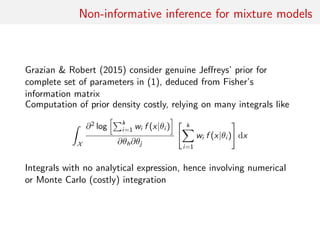
Jeffreys’ prior for mixture not available due to computational
reasons : it has not been tested so far
[Jeffreys, 1939]
Warning: Jeffreys’ prior improper in some settings
[Grazian & Robert, 2015]

6. Non-informative inference for mixture models
Grazian & Robert (2015) consider genuine Jeffreys’ prior for
complete set of parameters in (1), deduced from Fisher’s
information matrix
Computation of prior density costly, relying on many integrals like
ˆ
X
∂2
log
k
i=1 wi f (x|θi )
∂θh∂θj
k
i=1
wi f (x|θi ) dx
Integrals with no analytical expression, hence involving numerical
or Monte Carlo (costly) integration

7. Non-informative inference for mixture models
When building Metropolis-Hastings proposal over (wi , θi )’s, prior
ratio more expensive than likelihood and proposal ratios
Suggestion: split the acceptance rule
α(x, y) := 1 ∧ r(x, y), r(x, y) :=
π(y|D)q(y, x)
π(x|D)q(x, y)
into
˜α(x, y) := 1 ∧
f (D|y)q(y, x)
f (D|x)q(x, y)
× 1 ∧
π(y)
π(x)

8. The “Big Data” plague
Simulation from posterior distribution with large sample size n
• Computing time at least of order O(n)
• solutions using likelihood decomposition
n
i=1
(θ|xi )
and handling subsets on different processors (CPU), graphical
units (GPU), or computers
[Korattikara et al. (2013), Scott et al. (2013)]
• no consensus on method of choice, with instabilities from
removing most prior input and uncalibrated approximations
[Neiswanger et al. (2013), Wang and Dunson (2013)]

9. Proposed solution
“There is no problem an absence of decision cannot
solve.” Anonymous
1 Motivating example
2 Proposed solution
3 Validation of the method
4 Optimizing DA

10. Delayed acceptance
Given α(x, y) := 1 ∧ r(x, y), factorise
r(x, y) =
d
k=1
ρk(x, y)
under constraint ρk(x, y) = ρk(y, x)−1
Delayed Acceptance Markov kernel given by
˜P(x, A) :=
ˆ
A
q(x, y)˜α(x, y)dy + 1 −
ˆ
X
q(x, y)˜α(x, y)dy 1A(x)
where
˜α(x, y) :=
d
k=1
{1 ∧ ρk(x, y)}.

11. Delayed acceptance
Algorithm 1 Delayed Acceptance
To sample from ˜P(x, ·):
1 Sample y ∼ Q(x, ·).
2 For k = 1, . . . , d:
• with probability 1 ∧ ρk (x, y) continue
• otherwise stop and output x
3 Output y
Arrange terms in product so that most computationally intensive
ones calculated ‘at the end’ hence least often

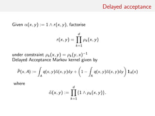
12. Delayed acceptance
Algorithm 1 Delayed Acceptance
To sample from ˜P(x, ·):
1 Sample y ∼ Q(x, ·).
2 For k = 1, . . . , d:
• with probability 1 ∧ ρk (x, y) continue
• otherwise stop and output x
3 Output y
Generalization of Fox and Nicholls (1997) and Christen and Fox
(2005), where testing for acceptance with approximation before
computing exact likelihood first suggested
More recent occurences in literature
[Golightly et al. (2014), Shestopaloff and Neal (2013)]

13. Potential drawbacks
• Delayed Acceptance efficiently reduces computing cost only
when approximation ˜π is “good enough” or “flat enough”
• Probability of acceptance always smaller than in the original
Metropolis–Hastings scheme
• Decomposition of original data in likelihood bits may however
lead to deterioration of algorithmic properties without
impacting computational efficiency...
• ...e.g., case of a term explosive in x = 0 and computed by
itself: leaving x = 0 near impossible

14. Potential drawbacks
Figure : (left) Fit of delayed Metropolis–Hastings algorithm on a
Beta-binomial posterior p|x ∼ Be(x + a, n + b − x) when N = 100,
x = 32, a = 7.5 and b = .5. Binomial B(N, p) likelihood replaced with
product of 100 Bernoulli terms. Histogram based on 105
iterations, with
overall acceptance rate of 9%; (centre) raw sequence of p’s in Markov
chain; (right) autocorrelogram of the above sequence.

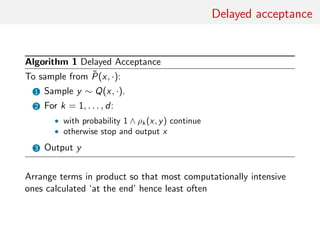
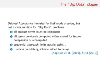
15. The “Big Data” plague
Delayed Acceptance intended for likelihoods or priors, but
not a clear solution for “Big Data” problems
1 all product terms must be computed
2 all terms previously computed either stored for future
comparison or recomputed
3 sequential approach limits parallel gains...
4 ...unless prefetching scheme added to delays
[Angelino et al. (2014), Strid (2010)]

16. Validation of the method
1 Motivating example
2 Proposed solution
3 Validation of the method
4 Optimizing DA

17. Validation of the method
Lemma (1)
For any Markov chain with transition kernel Π of the form
Π(x, A) =
ˆ
A
q(x, y)a(x, y)dy + 1 −
ˆ
X
q(x, y)a(x, y)dy 1A(x),
and satisfying detailed balance, the function a(·) satisfies (for
π-a.e. x, y)
a(x, y)
a(y, x)
= r(x, y).

18. Validation of the method
Lemma (2)
( ˜Xn)n≥1, the Markov chain associated with ˜P, is a π-reversible
Markov chain.
Proof.
From Lemma 1 we just need to check that
˜α(x, y)
˜α(y, x)
=
d
k=1
1 ∧ ρk(x, y)
1 ∧ ρk(y, x)
=
d
k=1
ρk(x, y) = r(x, y),
since ρk(y, x) = ρk(x, y)−1 and (1 ∧ a)/(1 ∧ a−1) = a

19. Comparisons of P and ˜P
The acceptance probability ordering
˜α(x, y) =
d
k=1
{1∧ρk(x, y)} ≤ 1∧
d
k=1
ρk(x, y) = 1∧r(x, y) = α(x, y),
follows from (1 ∧ a)(1 ∧ b) ≤ (1 ∧ ab) for a, b ∈ R+.
Remark
By construction of ˜P,
var(f , P) ≤ var(f , ˜P)
for any f ∈ L2(X, π), using Peskun ordering (Peskun, 1973,
Tierney, 1998), since ˜α(x, y) ≤ α(x, y) for any (x, y) ∈ X2.

20. Comparisons of P and ˜P
Condition (1)
Defining A := {(x, y) ∈ X2 : r(x, y) ≥ 1}, there exists c such that
inf(x,y)∈A mink∈{1,...,d} ρk(x, y) ≥ c.
Ensures that when
α(x, y) = 1
then acceptance probability ˜α(x, y) uniformly lower-bounded by
positive constant.
Reversibility implies ˜α(x, y) uniformly lower-bounded by a constant
multiple of α(x, y) for all x, y ∈ X.

21. Comparisons of P and ˜P
Condition (1)
Defining A := {(x, y) ∈ X2 : r(x, y) ≥ 1}, there exists c such that
inf(x,y)∈A mink∈{1,...,d} ρk(x, y) ≥ c.
Proposition (1)
Under Condition (1), Lemma 34 in Andrieu et al. (2013) implies
Gap ˜P ≥ Gap P and
var f , ˜P ≤ ( −1
− 1)varπ(f ) + −1
var (f , P)
with f ∈ L2
0(E, π), = cd−1.

22. Comparisons of P and ˜P
Proposition (1)
Under Condition (1), Lemma 34 in Andrieu et al. (2013) implies
Gap ˜P ≥ Gap P and
var f , ˜P ≤ ( −1
− 1)varπ(f ) + −1
var (f , P)
with f ∈ L2
0(E, π), = cd−1.
Hence if P has right spectral gap, then so does ˜P.
Plus, quantitative bounds on asymptotic variance of MCMC
estimates using ( ˜Xn)n≥1 in relation to those using (Xn)n≥1
available

23. Comparisons of P and ˜P
Easiest use of above: modify any candidate factorisation
Given factorisation of r
r(x, y) =
d
k=1
˜ρk(x, y) ,
satisfying the balance condition, define a sequence of functions ρk
such that both r(x, y) = d
k=1 ρk(x, y) and Condition 1 holds.

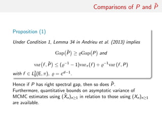
24. Comparisons of P and ˜P
Take c ∈ (0, 1], define b = c
1
d−1 and set
˜ρk(x, y) := min
1
b
, max {b, ρk(x, y)} , k ∈ {1, . . . , d − 1},
and
˜ρd (x, y) :=
r(x, y)
d−1
k=1 ˜ρk(x, y)
.
Then:
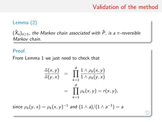
Proposition (2)
Under this scheme, previous proposition holds with
= c2
= b2(d−1)
.

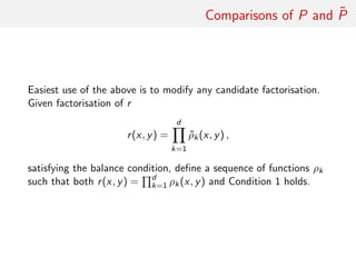
25. Proof of Proposition 1
optimising decomposition For any f ∈ L2(E, µ) define Dirichlet form
associated with a µ-reversible Markov kernel Π : E × B(E) as
EΠ(f ) :=
1
2
ˆ
µ(dx)Π(x, dy) [f (x) − f (y)]2
.
The (right) spectral gap of a generic µ-reversible Markov kernel
has the following variational representation
Gap (Π) := inf
f ∈L2
0(E,µ)
EΠ(f )
f , f µ
.

26. Proof of Proposition 1
optimising decomposition
Lemma (Andrieu et al., 2013, Lemma 34)
Let Π1 and Π2 be µ-reversible Markov transition kernels of
µ-irreducible and aperiodic Markov chains, and assume that there
exists > 0 such that for any f ∈ L2
0 E, µ
EΠ2 f ≥ EΠ1 f ,
then
Gap Π2 ≥ Gap Π1
and
var f , Π2 ≤ ( −1
− 1)varµ(f ) + −1
var (f , Π1) f ∈ L2
0(E, µ).

27. Optimizing delayed acceptance
1 Motivating example
2 Proposed solution
3 Validation of the method
4 Optimizing DA

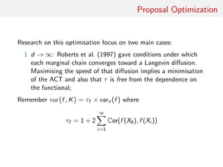
28. Proposal Optimisation
Explorative performances of random–walk MCMC strongly
dependent on proposal distribution
Finding optimal scale parameter leads to efficient ‘jumps’ in state
space and smaller...
1 expected square jump distance (ESJD)
2 overall acceptance rate (α)
3 asymptotic variance of ergodic average var f , K
[Roberts et al. (1997), Sherlock and Roberts (2009)]
Provides practitioners with ‘auto-tune’ version of resulting
random–walk MCMC algorithm

29. Proposal Optimisation
Quest for optimisation focussing on two main cases:
1 d → ∞: Roberts et al. (1997) give conditions under which
each marginal chain converges toward a Langevin diffusion
Maximising speed of that diffusion implies minimisation of the
ACT and also τ free from the functional
Remember var f , K = τf × varπ(f ) where
τf = 1 + 2
∞
i=1
Cor(f (X0), f (Xi ))

30. Proposal Optimisation
Quest for optimisation focussing on two main cases:
2 finite d: Sherlock and Roberts (2009) consider unimodal
elliptically symmetric targets and show proxy for ACT is
Expected Square Jumping Distance (ESJD), defined as
E X − X 2
β = E
d
i=1
β−2
i (Xi − X)2
As d → ∞, ESJD converges to the speed of the diffusion
process described in Roberts et al. (1997) [close asymptotia:
d 5]

31. Proposal Optimisation
“For a moment, nothing happened. Then, after a
second or so, nothing continued to happen.” —
D. Adams, THGG
When considering efficiency for Delayed Acceptance, focus on
execution time as well
Eff := ESJD cost per iteration
similar to Sherlock et al. (2013) for pseudo-Marginal MCMC

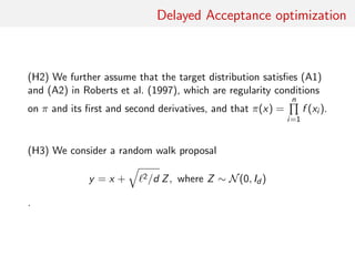
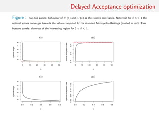
32. Delayed Acceptance optimisation
Set of assumptions:
(H1) Assume [for simplicity’s sake] that Delayed Acceptance
operates on two factors only, i.e.,
r(x, y) = ρ1(x, y) × ρ2(x, y),
˜α(x, y) =
2
i=1
(1 ∧ ρi (x, y))
Restriction also considers ideal setting where a computationally
cheap approximation ˜f (·) is available and precise enough so that
ρ2(x, y) = r(x, y)/ρ1(x, y) = π(y) π(x) × ˜f (x) ˜f (y) = 1
.

33. Delayed Acceptance optimisation
(H2) Assume that target distribution satisfies (A1) and (A2) in
Roberts et al. (1997), which are regularity conditions on π and its
first and second derivatives, and that
π(x) =
n
i=1
f (xi )
.
(H3) Consider only a random walk proposal
y = x + 2/d Z
where
Z ∼ N(0, Id )

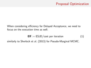
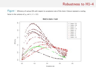
34. Delayed Acceptance optimisation
(H4) Assume that cost of computing ˜f (·), c say, proportional to
cost of computing π(·), C say, with c = δC.
Normalising by C = 1, average total cost per iteration of DA chain
is
δ + E [˜α]
and efficiency of proposed method under above conditions is
Eff(δ, ) =
ESJD
δ + E [˜α]

35. Delayed Acceptance optimisation
Lemma
Under conditions (H1)–(H4) on π(·), q(·, ·) and on
˜α(·, ·) = (1 ∧ ρ1(x, y))
As d → ∞
Eff(δ, ) ≈
h( )
δ + E [˜α]
=
2 2Φ(−
√
I/2)
δ + 2Φ(−
√
I/2)
a( ) ≈ E [˜α] = 2Φ(−
√
I/2)
where I := E ( π(x) )
π(x)
2
as in Roberts et al. (1997).

36. Delayed Acceptance optimisation
Proposition (3)
Under conditions of Lemma 3, optimal average acceptance rate
α∗(δ) is independent of I.
Proof.
Consider Eff(δ, ) in terms of (δ, a( )):
a = g( ) = 2Φ −
√
I/2 = g−1
(a) = −Φ−1
(a/2)
2
√
I
Eff(δ, a) =
4
I Φ−1 a
2
2
a
δ + a
=
4
I
1
δ + a
Φ−1 a
2
2
a

37. Delayed Acceptance optimisation
Figure : top panels: ∗
(δ) and α∗
(δ) as relative cost varies. For δ >> 1
the optimal values converges to values computed for the standard M-H
(red, dashed). bottom panels: close-up of interesting region for
0 < δ < 1.

38. Robustness wrt (H1)–(H4)
Figure : Efficiency of various DA wrt acceptance rate of the chain;
colours represent scaling factor in variance of ρ1 wrt π; δ = 0.3.

39. Practical optimisation
If computing cost comparable for all terms in
(x, y) =
K
i=1
ξi (x, y)
• rank entries according to the success rates observed on
preliminary run
• start with ratios with highest variances
• rank factors by correlation with full Metropolis–Hastings ratio

40. Illustrations
Logistic regression:
• 106 simulated observations with a 100-dimensional parameter
space
• optimised Metropolis–Hastings with α = 0.234
• DA optimised via empirical correlation
• split the data into subsamples of 10 elements
• include smallest number of subsamples to achieve 0.85
correlation
• optimise Σ against acceptance rate
algo ESS (av.) ESJD (av.)
DA-MH over MH 5.47 56.18

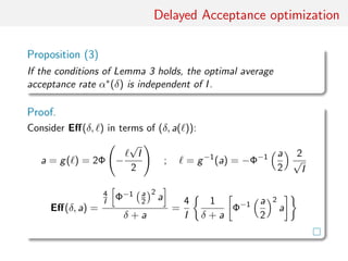
41. Illustrations
geometric MALA:
• proposal
θ = θ(i−1)
+ ε2
AT
A θ log(π(θ(i−1)
|y))/2 + εAυ
with position specific A
[Girolami and Calderhead (2011), Roberts and Stramer (2002)]
• computational bottleneck in computating 3rd derivative of π
in proposal
• G-MALA variance set to σ2
d =
2
d1/3
• 102 simulated observations with a 10-dimensional parameter
space
• DA optimised via acceptance rate
Eff(δ, a) = − (2/K)2/3 aΦ−1
(a/2)2/3
δ + a(1 − δ)
.
algo accept ESS/time (av.) ESJD/time (av.)
MALA 0.661 0.04 0.03
DA-MALA 0.09 0.35 0.31

42. Illustrations
Jeffreys for mixtures:
• numerical integration for each term in Fisher information
matrix
• split between likelihood (cheap) and prior (expensive) unstable
• saving 5% of the sample for second step
• MH and DA optimised via acceptance rate
• actual averaged gain ( ESSDA/ESSMH
timeDA/timeMH
) of 9.58
Algorithm ESS (aver.) ESJD (aver.) time (aver.)
MH 1575.963 0.226 513.95
MH + DA 628.767 0.215 42.22