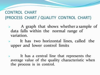
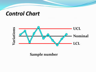
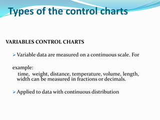
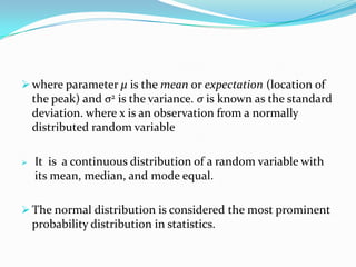
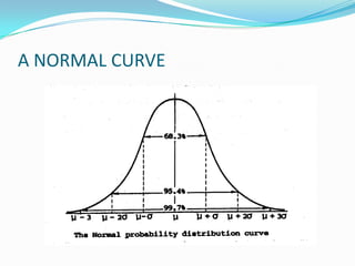
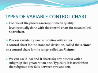
Statistical Quality Control (SQC) is used to evaluate organizational quality through statistical tools. SQC can be classified into descriptive statistics, statistical process control, and acceptance sampling. Descriptive statistics describe quality characteristics and relationships through measures like the mean and standard deviation. Statistical process control uses random sampling to determine if a process is producing products within a predetermined range. Acceptance sampling involves random inspection of samples to determine if an entire lot should be accepted or rejected. Control charts graphically show whether sample data falls within the normal variation limits.

2. Statistical Quality Control (SQC)
DEFINITION:
Statistical Quality Control is the term used to
describe the set of statistical tools to evaluate
organizational quality.
CLASSIFICATION OF SQC:
1.Descriptive statistics
2.Statistical process control
3.Acceptance sampling

3. DESCRIPTIVE STATISTICS
Statistics used to describe quality characteristics
and relationships.
Eg:
Mean, Standard deviation, Range

4. STATISTICAL PROCESS CONTROL
 A statistical tool that involve inspecting a
random sample of the output from a process and
deciding whether the process is producing
products with characteristics that fall within a
predetermined range.
 It answers the question whether the process
is functioning properly or not.

5. ACCEPTANCE SAMPLING
 The process of randomly inspecting
a sample of goods and deciding whether to accept
the entire lot based on the results.
 It determines whether a batch of
goods should be accepted or rejeted

6. VARIATION
It is the change in some quality
characteristic of the product or process.
CLASSIFICATION OF VARIATION:
1. In-control variation
2.Out-of-cotrol variation

7.  IN-CONTROL VARIATION:
Due to common causes(random causes)
that can’t be identified.
 OUT-OF-CONTROL VARIATION
Due to assignable causes(outside influences)
that can be identified and eliminated.

8. CONTROL CHART
(PROCESS CHART / QUALITY CONTROL CHART)
 A graph that shows whether a sample of
data falls within the normal range of
variation.
 It has two horizontal lines, called the
upper and lower control limits
 It has a central line that represents the
average value of the quality characteristic when
the process is in control.

9. Control Chart
UCL
Variations
Nominal
LCL
Sample number

10. Types of the control charts
VARIABLES CONTROL CHARTS
 Variable data are measured on a continuous scale. For
example:
time, weight, distance, temperature, volume, length,
width can be measured in fractions or decimals.
 Applied to data with continuous distribution

11. ATTRIBUTES CONTROL CHARTS
 Attribute data are counted and cannot have fractions or
decimals. Attribute data arise when you are determining only
the presence or absence of something.
 success or failure, accept or reject, correct or not correct.
Example:
a report can have four errors or five errors, but it cannot have
four and a half errors.
 Applied to data following discrete distribution

12. WHY CONTROL CHARTS ?
Predicting the expected range of outcomes from
a process.
Determining whether a process is stable (in
statistical control).
Analyzing patterns of process variation from
assignable causes or common causes .

13. PROCEDURE TO DRAW CONTROL
CHART
Choose the appropriate control chart for
the data.
Determine the appropriate time period
for collecting and plotting data.
Collect data, construct the chart and
analyze the data.
Look for “out-of-control signals” on the
control chart. When one is identified,
mark it on the chart and investigate the
cause.

14. General model for a control chart
UCL = μ + kσ
CL = μ
LCL = μ – kσ
where μ is the mean of the variable,and σ
is the standard deviation of the variable.
UCL=upper control limit;
LCL = lower control limit;
CL = center line.

15.  where k is the distance of the control
limits from the center line, expressed in
terms of standard deviation units
When k is set to 3, we speak of 3-sigma
control charts.

16. NORMAL DISTRIBUTION:
A variable control chart follows normal
distribution(since,variable is a continuous random variable)
A continuous random variable X having a
probability density function given by the formula
2
1 x
1 2
f ( x) e , x
2
is said to have a Normal Distribution with parameters
and 2. It is a theoretical distribution.
Symbolically, X ~ N( , 2). The distribution with μ = 0
and σ 2 = 1 is called the standard normal

17. Graph of generic normal
distribution

18.  where parameter μ is the mean or expectation (location of
the peak) and σ2 is the variance. σ is known as the standard
deviation. where x is an observation from a normally
distributed random variable
 It is a continuous distribution of a random variable with
its mean, median, and mode equal.
 The normal distribution is considered the most prominent
probability distribution in statistics.

19. PROPERTIES OF NORMAL DISTRIBUTION
1. The curve extends infinitely to the left and to the
right, approaching the x-axis as x increases in
magnitude, i.e. as x , f(x) 0.
2. The mode occurs at x= .
3. The curve is symmetric about a vertical axis through
the mean
4. The total area under the curve and above the
horizontal axis is equal to 1.
i.e.
2
1 x
1 2
e dx 1
2

20.  The mean identifies the position of the center and the
standard deviation determines the height and width of the
bell
 All normal density curves satisfy the following property
which is often referred to as the Empirical Rule or 68-95-
99.7 rule

21. EMPERICAL RULE:
 68% of the observations fall within 1 standard deviation
of the mean (i.e between μ -σ and μ + σ )
 95% of the observations fall within 2 standard deviations
of the mean (i.e between μ -2σ and μ + 2σ)
 99.7% of the observations fall within 3 standard
deviations of the mean(i.e between μ -3σ and μ +3σ)

22. A NORMAL CURVE

23. Eg:
 A good example of a bell curve or normal distribution
is the roll of two dice. The distribution is centered
around the number 7 and the probability decreases as
you move away from the center

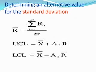
24. STANDARDIZING PROCESS
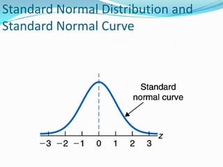
This can be done by means of the transformation.
The mean of Z is zero and the variance is respectively,
x
z
X
X Var( Z ) Var
E (Z ) E
1
2
Var( X )
1
E X
1
2
Var( X )
1
[E( X ) ] 1 2
2
0
1

25. Standard Normal Distribution and
Standard Normal Curve

26. TYPES OF VARIABLE CONTROL CHART
 Control of the process average or mean quality
level is usually done with the control chart for mean called
xbar chart.
 Process variability can be monitor with either
a control chart for the standard deviation, called the s chart,
or a control chart for the range, called an R chart.
 We can use X-bar and R charts for any process with a
subgroup size greater than one. Typically, it is used when
the subgroup size falls between two and ten,

27. Determining an alternative value
for the standard deviation
m
Ri
i 1
R
m
UCL X A2 R
LCL X A2 R

28. x-bar Chart Example: Unknown
OBSERVATIONS (SLIP- RING DIAMETER, CM)
SAMPLE k 1 2 3 4 5 x R
1 5.02 5.01 4.94 4.99 4.96 4.98 0.08
2 5.01 5.03 5.07 4.95 4.96 5.00 0.12
3 4.99 5.00 4.93 4.92 4.99 4.97 0.08
4 5.03 4.91 5.01 4.98 4.89 4.96 0.14
5 4.95 4.92 5.03 5.05 5.01 4.99 0.13
6 4.97 5.06 5.06 4.96 5.03 5.01 0.10
7 5.05 5.01 5.10 4.96 4.99 5.02 0.14
8 5.09 5.10 5.00 4.99 5.08 5.05 0.11
9 5.14 5.10 4.99 5.08 5.09 5.08 0.15
10 5.01 4.98 5.08 5.07 4.99 5.03 0.10
Totals 50.09 1.15
Copyright 2011 John Wiley & Sons, Inc. 3-38

29. 5.10 –
x- bar 5.08 –
Chart 5.06 –
UCL = 5.08
Example 5.04 –
5.02 – = = 5.01
Mean x
5.00 –
4.98 –
4.96 –
4.94 – LCL = 4.94
4.92 –
| | | | | | | | | |
1 2 3 4 5 6 7 8 9 10
Sample number
Copyright 2011 John Wiley & Sons, Inc. 3-39

30. R-Chart Example
OBSERVATIONS (SLIP- RING DIAMETER, CM)
SAMPLE k 1 2 3 4 5 x R
1 5.02 5.01 4.94 4.99 4.96 4.98 0.08
2 5.01 5.03 5.07 4.95 4.96 5.00 0.12
3 4.99 5.00 4.93 4.92 4.99 4.97 0.08
4 5.03 4.91 5.01 4.98 4.89 4.96 0.14
5 4.95 4.92 5.03 5.05 5.01 4.99 0.13
6 4.97 5.06 5.06 4.96 5.03 5.01 0.10
7 5.05 5.01 5.10 4.96 4.99 5.02 0.14
8 5.09 5.10 5.00 4.99 5.08 5.05 0.11
9 5.14 5.10 4.99 5.08 5.09 5.08 0.15
10 5.01 4.98 5.08 5.07 4.99 5.03 0.10
Totals 50.09 1.15
Copyright 2011 John Wiley & Sons, Inc. 3-40

31. R- Chart
UCL = D4R LCL = D3R
R
R= k
Where
R = range of each sample
k = number of samples (sub groups)
Copyright 2011 John Wiley & Sons, Inc. 3-41

32. R-Chart Example
_
UCL = D4R = 2.11(0.115) = 0.243
_
LCL = D3R = 0(0.115) = 0
Retrieve chart factors D3 and D4
Copyright 2011 John Wiley & Sons, Inc. 3-42

33. R-Chart Example
0.28 –
0.24 –
UCL = 0.243
0.20 –
0.16 –
Range
R = 0.115
0.12 –
0.08 –
0.04 – LCL = 0
0– | | | | | | | | | |
1 2 3 4 5 6 7 8 9 10
Sample number
Copyright 2011 John Wiley & Sons, Inc. 3-43

34. THANK YOU…..