Downloaded 181 times

1. The document discusses statistical quality control (SQC) methods including statistical process control (SPC), descriptive statistics, acceptance sampling, control charts, process capability analysis, and six sigma. 2. SPC uses control charts to monitor quality characteristics and identify sources of variation. Descriptive statistics are used to describe data distributions and central tendencies. 3. Acceptance sampling randomly inspects batches to determine acceptance or rejection. Control charts like X-bar, P, and C charts help monitor different quality characteristics. 4. Process capability analysis compares process variation to specification limits using metrics like Cp and Cpk. Six sigma aims for very low defect levels.


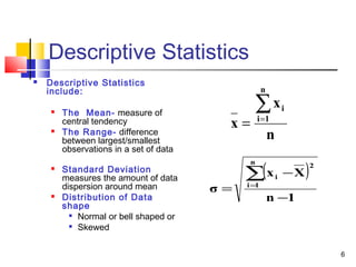
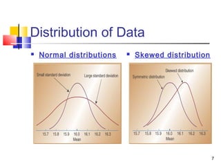
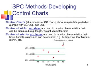
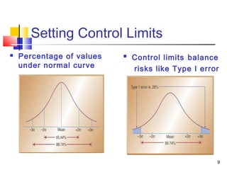
![Control Charts[1]](https://cdn.slidesharecdn.com/ss_thumbnails/controlcharts1-1226081330857138-9-thumbnail.jpg?width=640&height=640&fit=bounds)