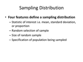
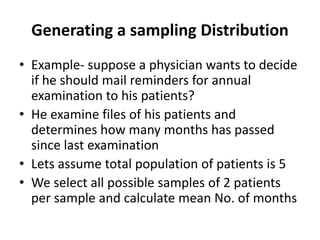
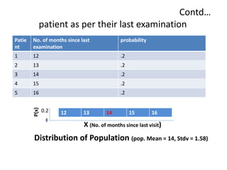
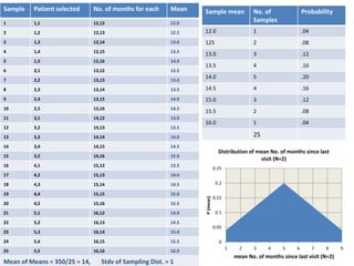
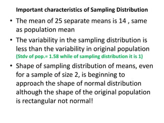
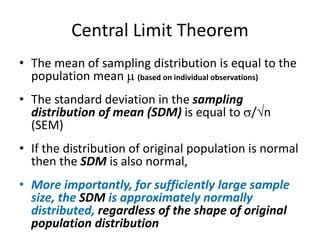
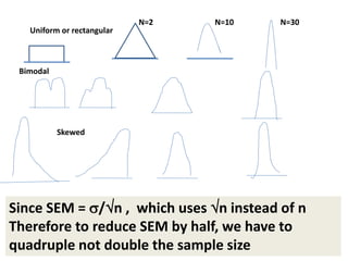
This document discusses sampling distributions and their use in making statistical inferences from data. It begins by defining key aspects of sampling distributions, including the statistic of interest (e.g. mean, proportion), random selection of samples, sample size, and population. It then generates a sampling distribution using an example of calculating the mean number of months since patients' last medical examination across different samples. The document outlines important characteristics of sampling distributions and how the central limit theorem applies. It also discusses how to construct confidence intervals and conduct hypothesis testing using sampling distributions.


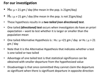


![ONFH[AVN HIP] -TRIPLE REGIME -A NOVAL SURGICAL CONCEPT .pptx](https://cdn.slidesharecdn.com/ss_thumbnails/onfhavnhip2026koaconcalicutdrgokuldevdrmashraf-260210064517-213ec005-thumbnail.jpg?width=640&height=640&fit=bounds)


![PERI-PROSTHETIC FRACTURE NAIL-PLATE CONSTRUCT [NPC].pptx](https://cdn.slidesharecdn.com/ss_thumbnails/drarunkumardrmohamedashrafperiprostheticfrasturenail-plateconstructnpc-260209164459-7e9d15a1-thumbnail.jpg?width=640&height=640&fit=bounds)