engineering mathematics

1. Statistics
Further Math
REVIEW CHAPTER
Normal distribution
Dr. KhoeYao Tung, MSc.Ed., M.Ed.

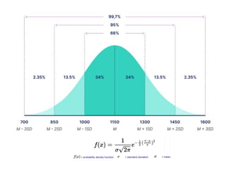
4. The normal is a family of
 Bell-shaped and symmetric distributions. because
the distribution is symmetric, one-half (.50 or
50%) lies on either side of the mean.
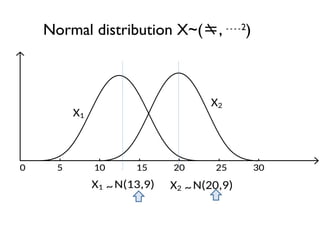
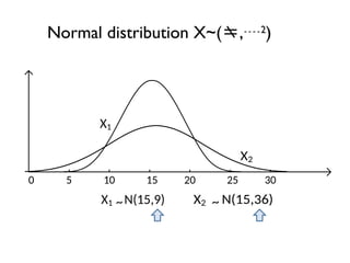
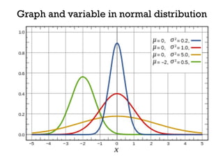
 Each is characterized by a different pair of mean
, and the variance, ² That is: [X~N(, ²)].
 Each is asymptotic to the horizontal axis.
Normal distribution

5. Normal distribution X~(, 2
)
5 10 15 20 25 30
X1 ~N(13,9)
X1
0
X2 ~N(20,9)
X2

6. Normal distribution X~(,2
)
5 10 15 20 25 30
X1 ~N(15,9)
X1
0
X2 ~ N(15,36)
X2

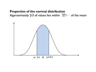
7. Properties of the normal distribution
Approximately 2/3 of values lies within 1 of the mean
(68.27%)
  


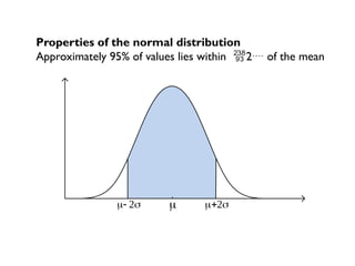
8. Properties of the normal distribution
Approximately 95% of values lies within 2 of the mean
(95.45%)
  


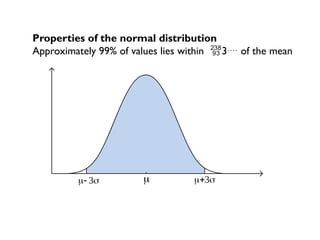
9. Properties of the normal distribution
Approximately 99% of values lies within 3 of the mean
(99.73%)
  


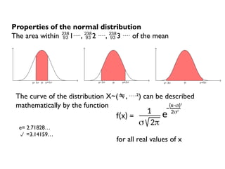
10. Properties of the normal distribution
The area within 1, 2 , 3  of the mean
The curve of the distribution X~(, ²) can be described
mathematically by the function
f(x) =
s 2p
1 e 2s2
(x- )2
s
for all real values of x
e= 2.71828…
 =3.14159…
  
   
   


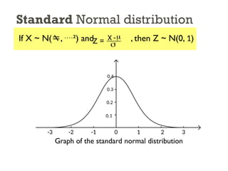
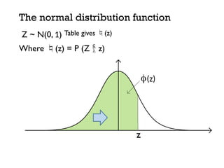
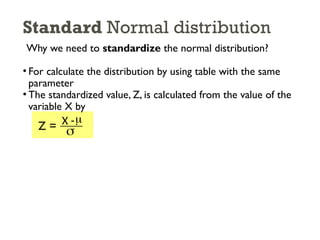
11. Standard Normal distribution
Why we need to standardize the normal distribution?
• For calculate the distribution by using table with the same
parameter
• The standardized value, Z, is calculated from the value of the
variable X by
Z = X -
s
m

12. Standard Normal distribution
If X ~ N(, ²) and , then Z ~ N(0, 1)
Z = X -
s
m
-2 -1 0 1 2 3
Graph of the standard normal distribution
-3
0.1
0.2
0.3
0.4

13. 0
Y


-
X

-  
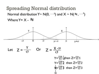
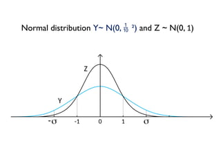
Spreading Normal distribution
Normal distributionY~ N(0, ²) and X ~ N(, ²)
WhereY= X - 
Let Z =
Y
s Or Z = X -
s
m
then Z=1
Y=
then Z=2
Y=2
 then Z=3
Y=3


14. Normal distribution Y~ N(0,  ²) and Z ~ N(0, 1)
-1 0 1
Z
Y


-

15. The normal distribution function
z
f(z)
Table gives (z)
Where (z) = P (Z  z)
Z ~ N(0, 1)

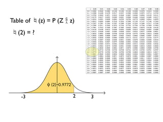
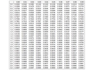
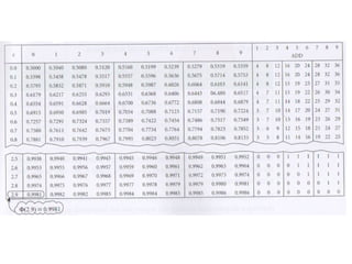
16. Table of (z) = P (Z  z)
(2) = ?
2
f (2)=0.9772
3
-3

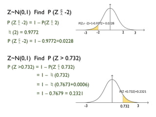
19. Z~N(0,1) Find P (Z  -2)
(2) = 0.9772
P (Z  -2) = 1 – P(Z  2)
Z~N(0,1) Find P (Z > 0.732)
P (Z >0.732) = 1 – P(Z  0.732)
= 1 – (0.732)
= 1 – (0.7673+0.0006)
= 1 – 0.7679 = 0.2321
P(Z < -2)=1-0.9772
-2
= 0.0228
2 3
-3
0.732 3
-3
P(Z >0.732)=0.2321
P (Z  -2) = 1 – 0.9772=0.0228

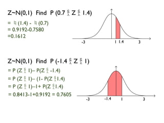
20. Z~N(0,1) Find P (0.7  Z  1.4)
= (1.4) - (0.7)
= 0.9192-0.7580
=0.1612
= P (Z  1)– P(Z  -1.4)
1.4 3
-3 1
Z~N(0,1) Find P (-1.4  Z  1)
= P (Z  1)– (1- P(Z 1.4)
= P (Z  1)–1+ P(Z 1.4)
= 0.8413-1+0.9192 = 0.7605
-1.4 3
-3 1

21. 2
0.7
3
-3 z
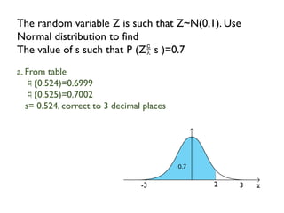
The random variable Z is such that Z~N(0,1). Use
Normal distribution to find
The value of s such that P (Z s )=0.7
a. From table
(0.524)=0.6999
(0.525)=0.7002
s= 0.524, correct to 3 decimal places

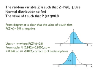
22. The random variable Z is such that Z~N(0,1). Use
Normal distribution to find
The value of t such that P (z>t)=0.8
From diagram it is clear that the value of t such that
P(Z>t)= 0.8 is negative
Use t = -v where P(Zv)=0.8
From table (0.842)=0.8000, so v
= 0.842 so t= -0.842, correct to 3 decimal places
t
0.8
3
-3 z
v
0.8
3
-3 z

23. Graph and variable in normal distribution

24. Standard Normal distribution
Why we need to standardize the normal distribution?
• For calculate the distribution by using table with the same
parameter
• The standardized value, Z, is calculated from the value of the
variable X by
Z = X -
s
m

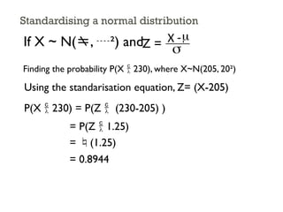
25. Standardising a normal distribution
If X ~ N(, ²) andZ = X -
s
m
Finding the probability P(X  230), where X~N(205, 20²)
Using the standarisation equation, Z= (X-205)
P(X  230) = P(Z  (230-205) )
= P(Z  1.25)
= (1.25)
= 0.8944

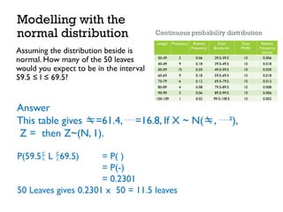
26. Modelling with the
normal distribution
Assuming the distribution beside is
normal. How many of the 50 leaves
would you expect to be in the interval
59.5 ≤ l ≤ 69.5?
Answer
This table gives =61.4, =16.8, If X ~ N(, ²),
Z = then Z~(N, 1).
P(59.5 L 69.5) = P( )
= P(-)
= 0.2301
50 Leaves gives 0.2301 x 50 = 11.5 leaves

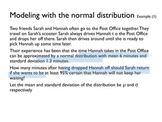
27. Modeling with the normal distribution Example (1)
Two friends Sarah and Hannah often go to the Post Office together.They
travel on Sarah’s scooter. Sarah always drives Hannah t o the Post Office
and drops her off there. Sarah then drives around until she is ready to
pick Hannah up some time later.
Their experience has been that the time Hannah takes in the Post Office
can be approximated by a normal distribution with mean 6 minutes and
standard deviation 1.3 minutes.
How many minutes after having dropped Hannah off should Sarah return
if she wants to be at least 95% certain that Hannah will not keep her
waiting?
Let the mean and standard deviation of the distribution be and
μ σ
respectively

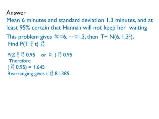
28. This problem gives =6, =1.3, then T~ N(6, 1.3²),
Find P(T  t) 
P(Z   0.95 or  (  0.95
Therefore
(  0.95) = 1.645
Rearranging gives t  8.1385
Answer
Mean 6 minutes and standard deviation 1.3 minutes, and at
least 95% certain that Hannah will not keep her waiting

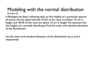
29. A Biologist has been collecting data on the heights of a particular species
of cactus. He has observed that 34.2% of the cacti are below 12 cm in
height and 18.4% of the cacti are above 16 cm in height. He assumes that
the heights are normally distributed. Find the mean and standard deviation
of the distribution.
Let the mean and standard deviation of the distribution be and
μ σ
respectively
Modeling with the normal distribution
Example (2)

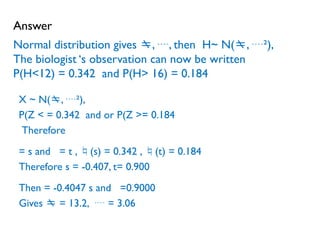
30. Normal distribution gives , , then H~ N(, ²),
The biologist ‘s observation can now be written
P(H<12) = 0.342 and P(H> 16) = 0.184
X ~ N(, ²),
P(Z < = 0.342 and or P(Z >= 0.184
Therefore
= s and = t , (s) = 0.342 , (t) = 0.184
Therefore s = -0.407, t= 0.900
Then = -0.4047 s and =0.9000
Gives  = 13.2,  = 3.06
Answer

31. 5 10 15
n=12, p=0.1
5 10 15
n=20, p=0.1
5 10 15
n=60, p=0.1
Approximation to binomial distribution
4 8 12
n=12, p=0.5
5 10 20
n=20, p=0.5
20 30 60
n=60, p=0.5
40 50
10
15

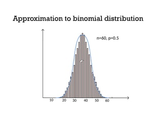
32. 20 30 60
n=60, p=0.5
40 50
10
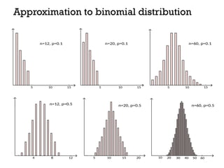
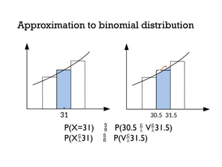
Approximation to binomial distribution

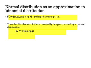
33. Normal distribution as an approximation to
binomial distribution
• If X~B(n,p), and if np>5 and nq>5, where q=1-p,
• Then the distribution of X can reasonably be approximated by a normal
distribution,
by V~N(np, npq)

34. Approximation to binomial distribution
31 30.5 31.5
P(X=31)  P(30.5  V31.5)
P(X31)  P(V31.5)

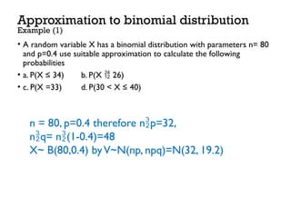
35. • A random variable X has a binomial distribution with parameters n= 80
and p=0.4 use suitable approximation to calculate the following
probabilities
• a. P(X ≤ 34) b. P(X  26)
• c. P(X =33) d. P(30 < X ≤ 40)
Approximation to binomial distribution
Example (1)
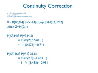
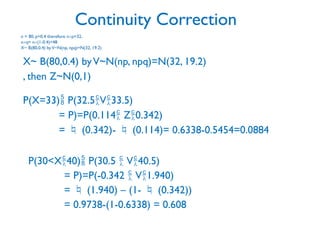
n = 80, p=0.4 therefore np=32,
nq= n(1-0.4)=48
X~ B(80,0.4) byV~N(np, npq)=N(32, 19.2)

36. X~ B(80,0.4) byV~N(np, npq)=N(32, 19.2)
, then Z~N(0,1)
P(X34) P(V34.5)
= P)=P(Z0.570…)
=  (0.571)= 0.716
P(X26) P(V  25.5)
= P)=P(Z  -1.483…)
= 1-  (1.483)= 0.931
Continuity Correction

37. X~ B(80,0.4) byV~N(np, npq)=N(32, 19.2)
, then Z~N(0,1)
P(X=33) P(32.5V33.5)
= P)=P(0.114 Z0.342)
=  (0.342)-  (0.114)= 0.6338-0.5454=0.0884
P(30<X40) P(30.5  V40.5)
= P)=P(-0.342  V1.940)
=  (1.940) – (1-  (0.342))
= 0.9738-(1-0.6338) = 0.608
Continuity Correction