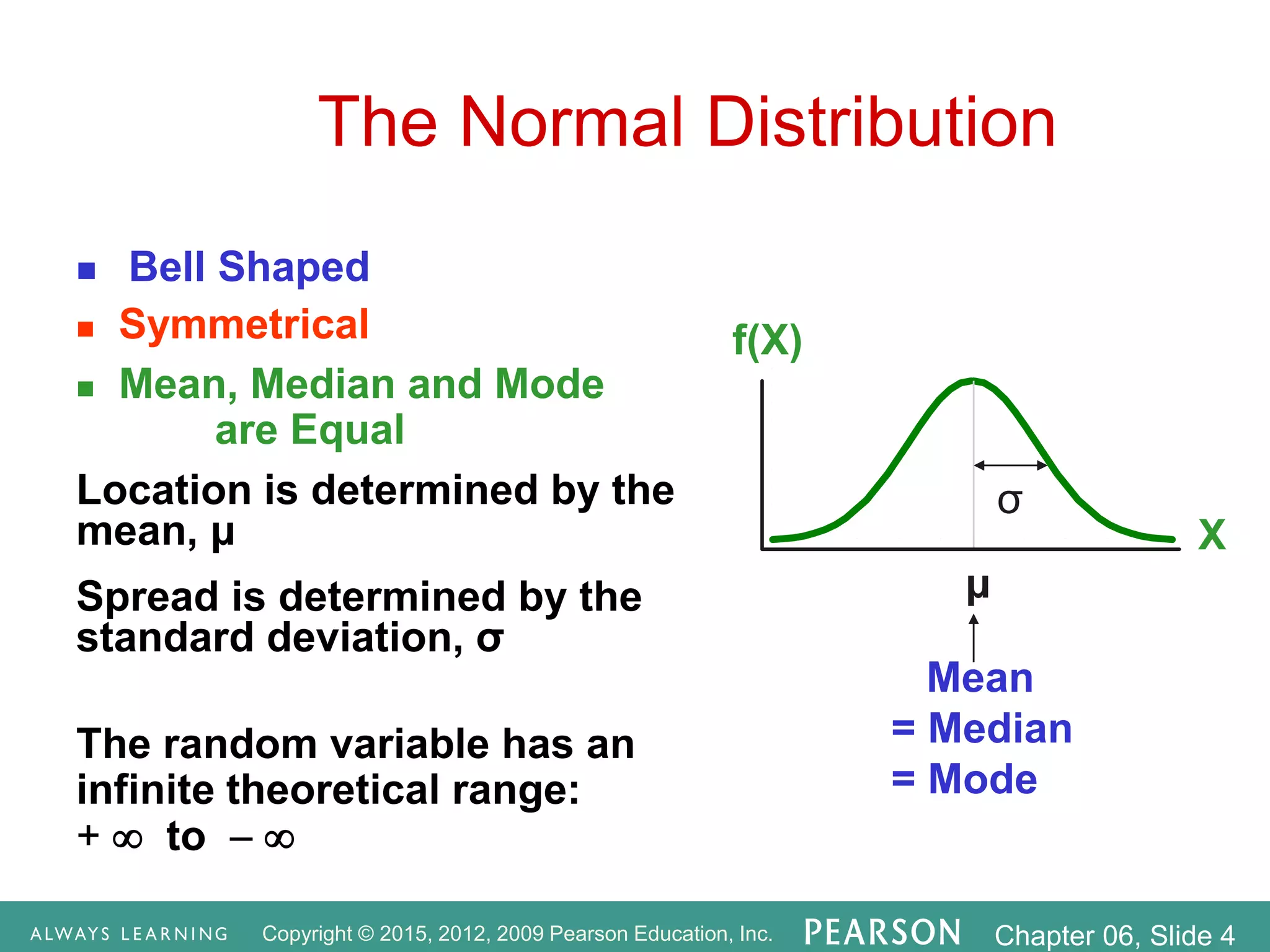
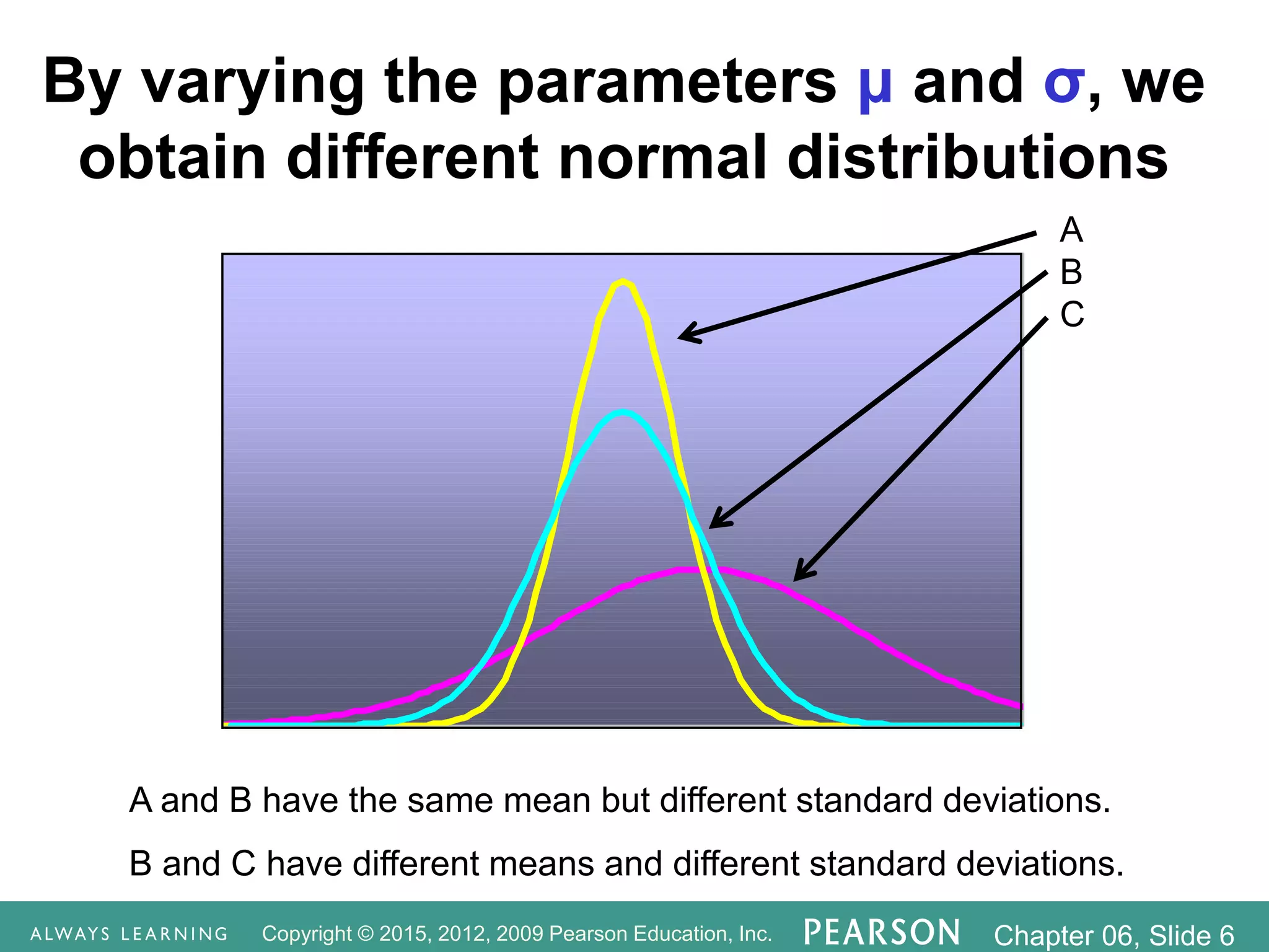
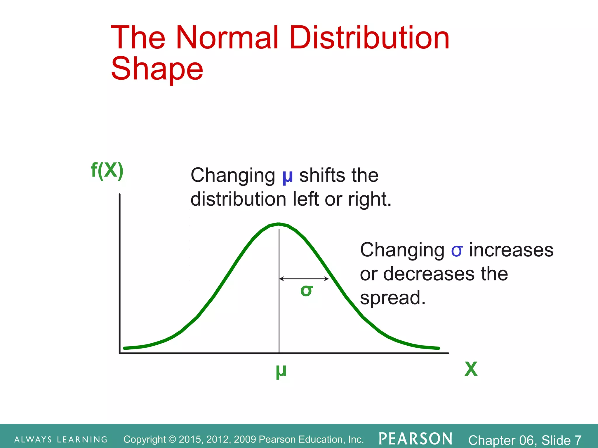
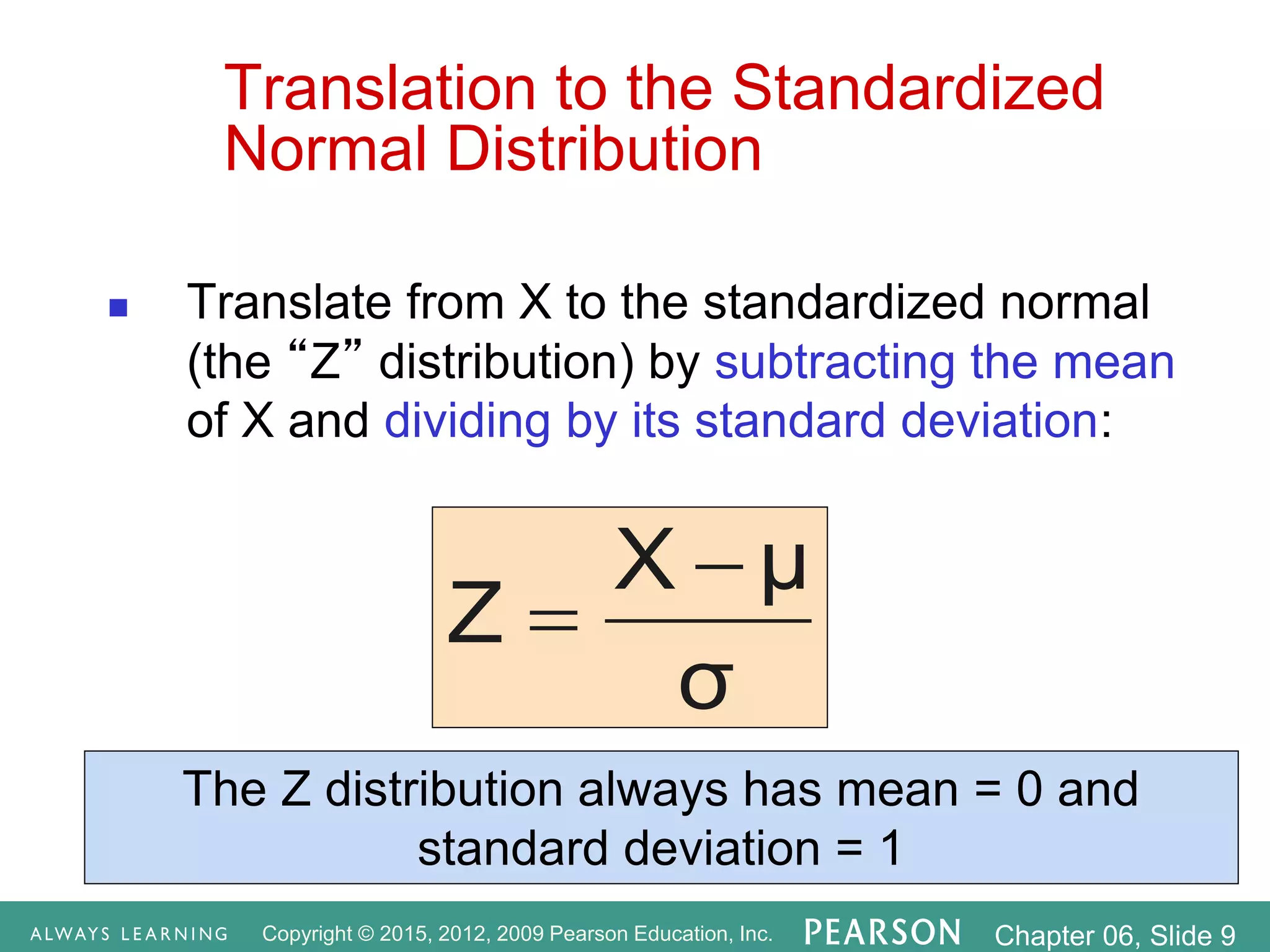
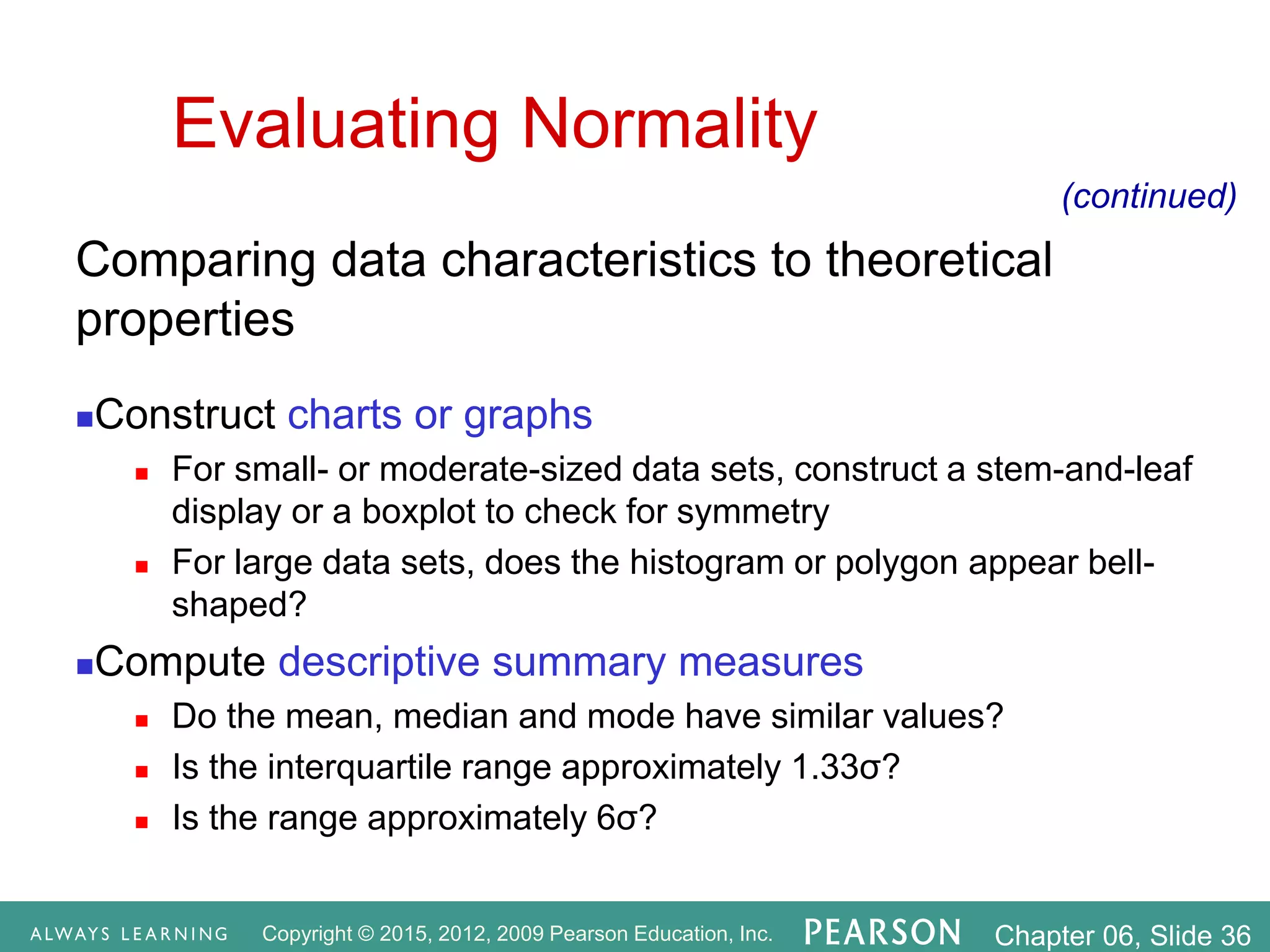
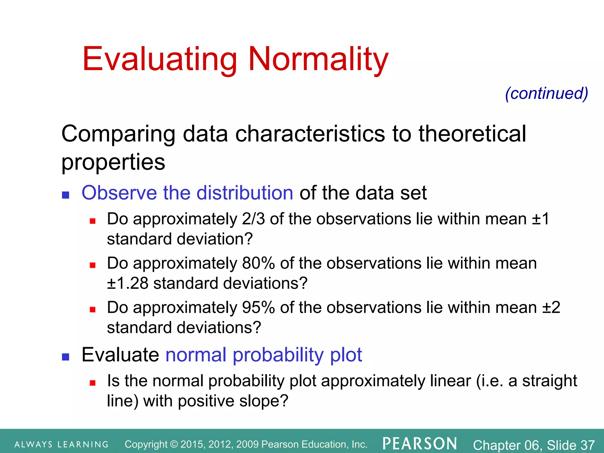
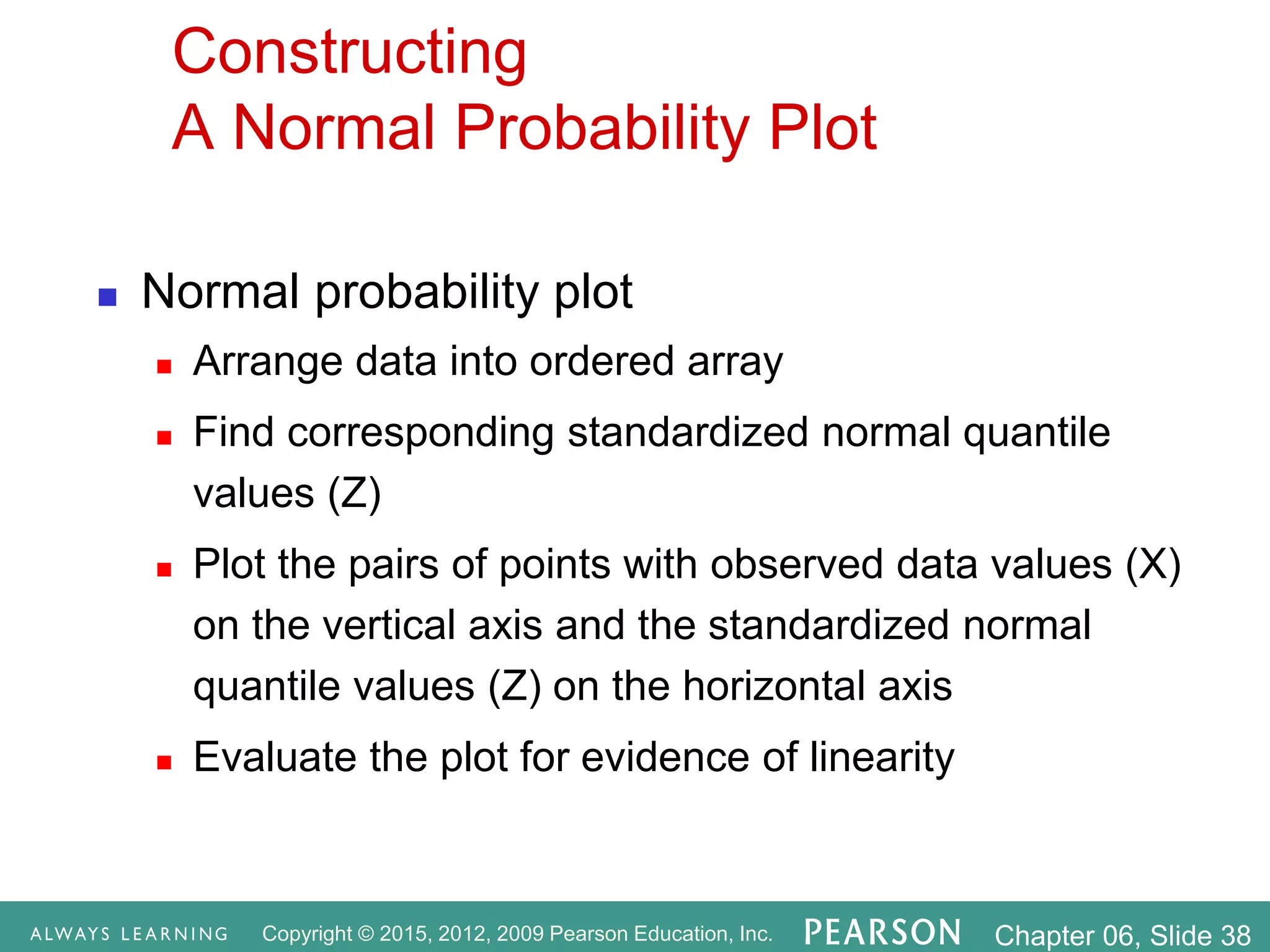
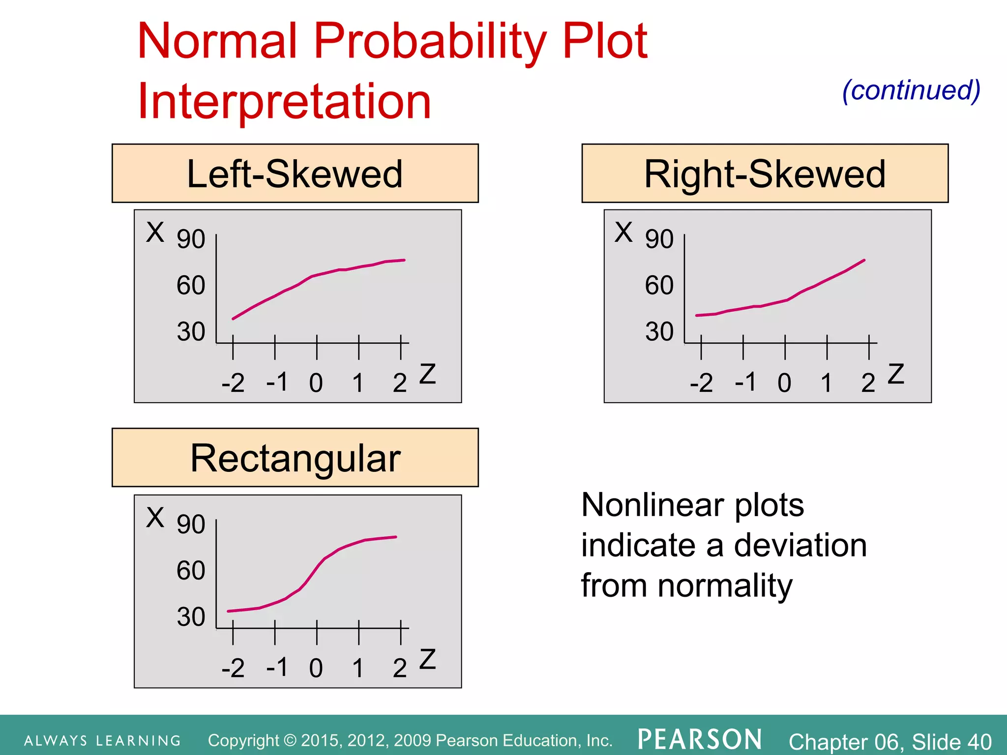
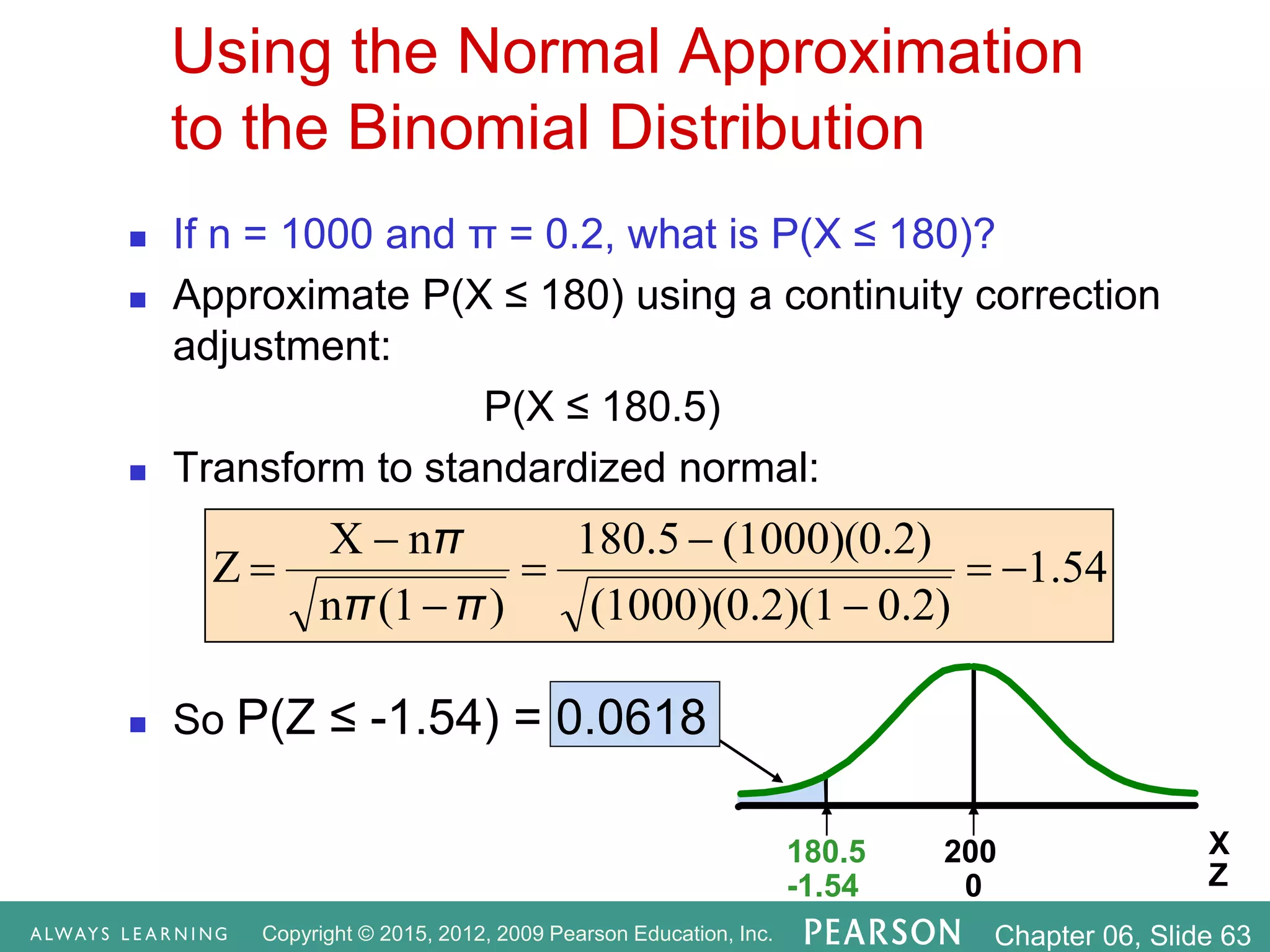
SlideShare a Scribd company logo
1 of 64
Copyright © 2015, 2012, 2009 Pearson Education, Inc. Chapter 06, Slide 1
The Normal Distribution
and Other Continuous
Distributions
Chapter 6
Copyright © 2015, 2012, 2009 Pearson Education, Inc. Chapter 06, Slide 2
Learning Objectives
In this chapter, you learn:
 To compute probabilities from the normal distribution
 How to use the normal distribution to solve business
problems
 To use the normal probability plot to determine whether
a set of data is approximately normally distributed
 To compute probabilities from the uniform distribution
 To compute probabilities from the exponential
distribution
Copyright © 2015, 2012, 2009 Pearson Education, Inc. Chapter 06, Slide 3
Continuous Probability Distributions
 A continuous random variable is a variable that
can assume any value on a continuum (can
assume an uncountable number of values)
 thickness of an item
 time required to complete a task
 temperature of a solution
 height, in inches
 These can potentially take on any value
depending only on the ability to precisely and
accurately measure
Copyright © 2015, 2012, 2009 Pearson Education, Inc. Chapter 06, Slide 4
The Normal Distribution
 ‘Bell Shaped’
 Symmetrical
 Mean, Median and Mode
are Equal
Location is determined by the
mean, μ
Spread is determined by the
standard deviation, σ
The random variable has an
infinite theoretical range:
+  to  
Mean
= Median
= Mode
X
f(X)
μ
σ
Copyright © 2015, 2012, 2009 Pearson Education, Inc. Chapter 06, Slide 5
The Normal Distribution
Density Function
2
μ)
(X
2
1
e
2π
1
f(X)





 

 

 The formula for the normal probability density function is
Where e = the mathematical constant approximated by 2.71828
π = the mathematical constant approximated by 3.14159
μ = the population mean
σ = the population standard deviation
X = any value of the continuous variable
Copyright © 2015, 2012, 2009 Pearson Education, Inc. Chapter 06, Slide 6
By varying the parameters μ and σ, we
obtain different normal distributions
A
B
C
A and B have the same mean but different standard deviations.
B and C have different means and different standard deviations.
Copyright © 2015, 2012, 2009 Pearson Education, Inc. Chapter 06, Slide 7
The Normal Distribution
Shape
X
f(X)
μ
σ
Changing μ shifts the
distribution left or right.
Changing σ increases
or decreases the
spread.
Copyright © 2015, 2012, 2009 Pearson Education, Inc. Chapter 06, Slide 8
The Standardized Normal
 Any normal distribution (with any mean and
standard deviation combination) can be
transformed into the standardized normal
distribution (Z)
 To compute normal probabilities need to
transform X units into Z units
 The standardized normal distribution (Z) has a
mean of 0 and a standard deviation of 1
Copyright © 2015, 2012, 2009 Pearson Education, Inc. Chapter 06, Slide 9
Translation to the Standardized
Normal Distribution
 Translate from X to the standardized normal
(the “Z” distribution) by subtracting the mean
of X and dividing by its standard deviation:
σ
μ
X
Z


The Z distribution always has mean = 0 and
standard deviation = 1
Copyright © 2015, 2012, 2009 Pearson Education, Inc. Chapter 06, Slide 10
The Standardized Normal
Probability Density Function
 The formula for the standardized normal
probability density function is
Where e = the mathematical constant approximated by 2.71828
π = the mathematical constant approximated by 3.14159
Z = any value of the standardized normal distribution
2
(1/2)Z
e
2π
1
f(Z) 

Copyright © 2015, 2012, 2009 Pearson Education, Inc. Chapter 06, Slide 11
The Standardized
Normal Distribution
 Also known as the “Z” distribution
 Mean is 0
 Standard Deviation is 1
Z
f(Z)
0
1
Values above the mean have positive Z-values.
Values below the mean have negative Z-values.
Copyright © 2015, 2012, 2009 Pearson Education, Inc. Chapter 06, Slide 12
Example
 If X is distributed normally with mean of $100
and standard deviation of $50, the Z value
for X = $200 is
 This says that X = $200 is two standard
deviations (2 increments of $50 units) above
the mean of $100.
2.0
$50
100
$
$200
σ
μ
X
Z 




Copyright © 2015, 2012, 2009 Pearson Education, Inc. Chapter 06, Slide 13
Comparing X and Z units
Note that the shape of the distribution is the same,
only the scale has changed. We can express the
problem in the original units (X in dollars) or in
standardized units (Z)
Z
$100
2.0
0
$200 $X(μ = $100, σ = $50)
(μ = 0, σ = 1)
Copyright © 2015, 2012, 2009 Pearson Education, Inc. Chapter 06, Slide 14
Finding Normal Probabilities
a b X
f(X) P a X b
( )
≤
Probability is measured by the area
under the curve
≤
P a X b
( )
<
<
=
(Note that the
probability of any
individual value is zero)
Copyright © 2015, 2012, 2009 Pearson Education, Inc. Chapter 06, Slide 15
f(X)
X
μ
Probability as
Area Under the Curve
0.5
0.5
The total area under the curve is 1.0, and the curve is
symmetric, so half is above the mean, half is below
1.0
)
X
P( 




0.5
)
X
P(μ 



0.5
μ)
X
P( 



Copyright © 2015, 2012, 2009 Pearson Education, Inc. Chapter 06, Slide 16
The Standardized Normal Table
 The Cumulative Standardized Normal table
in the textbook (Appendix table E.2) gives the
probability less than a desired value of Z (i.e.,
from negative infinity to Z)
Z
0 2.00
0.9772
Example:
P(Z < 2.00) = 0.9772
Copyright © 2015, 2012, 2009 Pearson Education, Inc. Chapter 06, Slide 17
The Standardized Normal Table
The value within the
table gives the
probability from Z =  
up to the desired Z
value
.9772
2.0
P(Z < 2.00) = 0.9772
The row shows
the value of Z
to the first
decimal point
The column gives the value of
Z to the second decimal point
2.0
.
.
.
(continued)
Z 0.00 0.01 0.02 …
0.0
0.1
Copyright © 2015, 2012, 2009 Pearson Education, Inc. Chapter 06, Slide 18
General Procedure for
Finding Normal Probabilities
 Draw the normal curve for the problem in
terms of X
 Translate X-values to Z-values
 Use the Standardized Normal Table
To find P(a < X < b) when X is
distributed normally:
Copyright © 2015, 2012, 2009 Pearson Education, Inc. Chapter 06, Slide 19
Finding Normal Probabilities
 Let X represent the time it takes (in seconds)
to download an image file from the internet.
 Suppose X is normal with a mean of18.0
seconds and a standard deviation of 5.0
seconds. Find P(X < 18.6)
18.6
X
18.0
Copyright © 2015, 2012, 2009 Pearson Education, Inc. Chapter 06, Slide 20
 Let X represent the time it takes, in seconds to download an image file
from the internet.
 Suppose X is normal with a mean of 18.0 seconds and a standard
deviation of 5.0 seconds. Find P(X < 18.6)
Z
0.12
0
X
18.6
18
μ = 18
σ = 5
μ = 0
σ = 1
(continued)
Finding Normal Probabilities
0.12
5.0
8.0
1
18.6
σ
μ
X
Z 




P(X < 18.6) P(Z < 0.12)
Copyright © 2015, 2012, 2009 Pearson Education, Inc. Chapter 06, Slide 21
Z
0.12
Z .00 .01
0.0 .5000 .5040 .5080
.5398 .5438
0.2 .5793 .5832 .5871
0.3 .6179 .6217 .6255
Solution: Finding P(Z < 0.12)
0.5478
.02
0.1 .5478
Standardized Normal Probability
Table (Portion)
0.00
= P(Z < 0.12)
P(X < 18.6)
Copyright © 2015, 2012, 2009 Pearson Education, Inc. Chapter 06, Slide 22
Finding Normal
Upper Tail Probabilities
 Suppose X is normal with mean 18.0
and standard deviation 5.0.
 Now Find P(X > 18.6)
X
18.6
18.0
Copyright © 2015, 2012, 2009 Pearson Education, Inc. Chapter 06, Slide 23
 Now Find P(X > 18.6)…
(continued)
Z
0.12
0
Z
0.12
0.5478
0
1.000 1.0 - 0.5478
= 0.4522
P(X > 18.6) = P(Z > 0.12) = 1.0 - P(Z ≤ 0.12)
= 1.0 - 0.5478 = 0.4522
Finding Normal
Upper Tail Probabilities
Copyright © 2015, 2012, 2009 Pearson Education, Inc. Chapter 06, Slide 24
Finding a Normal Probability
Between Two Values
 Suppose X is normal with mean 18.0 and
standard deviation 5.0. Find P(18 < X < 18.6)
P(18 < X < 18.6)
= P(0 < Z < 0.12)
Z
0.12
0
X
18.6
18
0
5
8
1
18
σ
μ
X
Z 




0.12
5
8
1
18.6
σ
μ
X
Z 




Calculate Z-values:
Copyright © 2015, 2012, 2009 Pearson Education, Inc. Chapter 06, Slide 25
Z
0.12
Solution: Finding P(0 < Z < 0.12)
0.0478
0.00
= P(0 < Z < 0.12)
P(18 < X < 18.6)
= P(Z < 0.12) – P(Z ≤ 0)
= 0.5478 - 0.5000 = 0.0478
0.5000
Z .00 .01
0.0 .5000 .5040 .5080
.5398 .5438
0.2 .5793 .5832 .5871
0.3 .6179 .6217 .6255
.02
0.1 .5478
Standardized Normal Probability
Table (Portion)
Copyright © 2015, 2012, 2009 Pearson Education, Inc. Chapter 06, Slide 26
 Suppose X is normal with mean 18.0
and standard deviation 5.0.
 Now Find P(17.4 < X < 18)
X
17.4
18.0
Probabilities in the Lower Tail
Copyright © 2015, 2012, 2009 Pearson Education, Inc. Chapter 06, Slide 27
Probabilities in the Lower Tail
Now Find P(17.4 < X < 18)…
X
17.4 18.0
P(17.4 < X < 18)
= P(-0.12 < Z < 0)
= P(Z < 0) – P(Z ≤ -0.12)
= 0.5000 - 0.4522 = 0.0478
(continued)
0.0478
0.4522
Z
-0.12 0
The Normal distribution is
symmetric, so this probability
is the same as P(0 < Z < 0.12)
Copyright © 2015, 2012, 2009 Pearson Education, Inc. Chapter 06, Slide 28
Empirical Rule
μ ± 1σ encloses about
68.26% of X’s
f(X)
X
μ μ+1σ
μ-1σ
What can we say about the distribution of values
around the mean? For any normal distribution:
σ
σ
68.26%
Copyright © 2015, 2012, 2009 Pearson Education, Inc. Chapter 06, Slide 29
The Empirical Rule
 μ ± 2σ covers about 95.44% of X’s
 μ ± 3σ covers about 99.73% of X’s
x
μ
2σ 2σ
x
μ
3σ 3σ
95.44% 99.73%
(continued)
Copyright © 2015, 2012, 2009 Pearson Education, Inc. Chapter 06, Slide 30
 Steps to find the X value for a known
probability:
1. Find the Z value for the known probability
2. Convert to X units using the formula:
Given a Normal Probability
Find the X Value
Zσ
μ
X 

Copyright © 2015, 2012, 2009 Pearson Education, Inc. Chapter 06, Slide 31
Finding the X value for a
Known Probability
Example:
 Let X represent the time it takes (in seconds) to
download an image file from the internet.
 Suppose X is normal with mean 18.0 and standard
deviation 5.0
 Find X such that 20% of download times are less than
X.
X
? 18.0
0.2000
Z
? 0
(continued)
Copyright © 2015, 2012, 2009 Pearson Education, Inc. Chapter 06, Slide 32
Find the Z value for
20% in the Lower Tail
 20% area in the lower
tail is consistent with a
Z value of -0.84
Z .03
-0.9 .1762 .1736
.2033
-0.7 .2327 .2296
.04
-0.8 .2005
Standardized Normal Probability
Table (Portion)
.05
.1711
.1977
.2266
…
…
…
…
X
? 18.0
0.2000
Z
-0.84 0
1. Find the Z value for the known probability
Copyright © 2015, 2012, 2009 Pearson Education, Inc. Chapter 06, Slide 33
2. Convert to X units using the formula:
Finding the X value
8
.
13
0
.
5
)
84
.
0
(
0
.
18
Zσ
μ
X






So 20% of the values from a distribution
with mean 18.0 and standard deviation
5.0 are less than 13.80
Copyright © 2015, 2012, 2009 Pearson Education, Inc. Chapter 06, Slide 34
Both Minitab & Excel Can Be Used
To Find Normal Probabilities
Find P(X < 9) where X is normal with a mean of 7
and a standard deviation of 2
Excel Minitab
Copyright © 2015, 2012, 2009 Pearson Education, Inc. Chapter 06, Slide 35
Evaluating Normality
 Not all continuous distributions are normal
 It is important to evaluate how well the data set is
approximated by a normal distribution.
 Normally distributed data should approximate the
theoretical normal distribution:
 The normal distribution is bell shaped (symmetrical)
where the mean is equal to the median.
 The empirical rule applies to the normal distribution.
 The interquartile range of a normal distribution is 1.33
standard deviations.
Copyright © 2015, 2012, 2009 Pearson Education, Inc. Chapter 06, Slide 36
Evaluating Normality
Comparing data characteristics to theoretical
properties
Construct charts or graphs
 For small- or moderate-sized data sets, construct a stem-and-leaf
display or a boxplot to check for symmetry
 For large data sets, does the histogram or polygon appear bell-
shaped?
Compute descriptive summary measures
 Do the mean, median and mode have similar values?
 Is the interquartile range approximately 1.33σ?
 Is the range approximately 6σ?
(continued)
Copyright © 2015, 2012, 2009 Pearson Education, Inc. Chapter 06, Slide 37
Evaluating Normality
Comparing data characteristics to theoretical
properties
 Observe the distribution of the data set
 Do approximately 2/3 of the observations lie within mean ±1
standard deviation?
 Do approximately 80% of the observations lie within mean
±1.28 standard deviations?
 Do approximately 95% of the observations lie within mean ±2
standard deviations?
 Evaluate normal probability plot
 Is the normal probability plot approximately linear (i.e. a straight
line) with positive slope?
(continued)
Copyright © 2015, 2012, 2009 Pearson Education, Inc. Chapter 06, Slide 38
Constructing
A Normal Probability Plot
 Normal probability plot
 Arrange data into ordered array
 Find corresponding standardized normal quantile
values (Z)
 Plot the pairs of points with observed data values (X)
on the vertical axis and the standardized normal
quantile values (Z) on the horizontal axis
 Evaluate the plot for evidence of linearity
Copyright © 2015, 2012, 2009 Pearson Education, Inc. Chapter 06, Slide 39
A normal probability plot for data
from a normal distribution will be
approximately linear:
30
60
90
-2 -1 0 1 2 Z
X
The Normal Probability Plot
Interpretation
Copyright © 2015, 2012, 2009 Pearson Education, Inc. Chapter 06, Slide 40
Normal Probability Plot
Interpretation
Left-Skewed Right-Skewed
Rectangular
30
60
90
-2 -1 0 1 2 Z
X
(continued)
30
60
90
-2 -1 0 1 2 Z
X
30
60
90
-2 -1 0 1 2 Z
X Nonlinear plots
indicate a deviation
from normality
Copyright © 2015, 2012, 2009 Pearson Education, Inc. Chapter 06, Slide 41
Evaluating Normality
An Example: Mutual Fund Returns
The boxplot is skewed to
the right. (The normal
distribution is symmetric.)
Copyright © 2015, 2012, 2009 Pearson Education, Inc. Chapter 06, Slide 42
Evaluating Normality
An Example: Mutual Fund Returns
Descriptive Statistics
(continued)
• The mean (21.84) is approximately the same as the median
(21.65). (In a normal distribution the mean and median are
equal.)
• The interquartile range of 6.98 is approximately 1.09 standard
deviations. (In a normal distribution the interquartile range is
1.33 standard deviations.)
• The range of 59.52 is equal to 9.26 standard deviations. (In a
normal distribution the range is 6 standard deviations.)
• 77.04% of the observations are within 1 standard deviation of
the mean. (In a normal distribution this percentage is 68.26%.
• 86.79% of the observations are within 1.28 standard
deviations of the mean. (In a normal distribution this
percentage is 80%.)
• 96.86% of the observations are within 2 standard deviations
of the mean. (In a normal distribution this percentage is
95.44%.)
• The skewness statistic is 1.698 and the kurtosis statistic is
8.467. (In a normal distribution, each of these statistics equals
zero.)
Copyright © 2015, 2012, 2009 Pearson Education, Inc. Chapter 06, Slide 43
Evaluating Normality Via Excel
An Example: Mutual Fund Returns
(continued)
Plot is not a straight
line and shows the
distribution is skewed
to the right. (The
normal distribution
appears as a straight
line.)
Excel (quantile-quantile) normal probability plot
Copyright © 2015, 2012, 2009 Pearson Education, Inc. Chapter 06, Slide 44
Evaluating Normality Via Minitab
An Example: Mutual Fund Returns
(continued)
Plot is not a straight
line, rises quickly in
the beginning, rises
slowly at the end and
shows the distribution
is skewed to the
right.
Normal Probability Plot From Minitab
70
60
50
40
30
20
10
0
99.9
99
95
90
80
70
60
50
40
30
20
10
5
1
0.1
3YrReturn%
Percent
Probability Plot of 3YrReturn%
Normal
Copyright © 2015, 2012, 2009 Pearson Education, Inc. Chapter 06, Slide 45
Evaluating Normality
An Example: Mutual Fund Returns
 Conclusions
 The returns are right-skewed
 The returns have more values concentrated around
the mean than expected
 The range is larger than expected
 Normal probability plot is not a straight line
 Overall, this data set greatly differs from the
theoretical properties of the normal distribution
(continued)
Copyright © 2015, 2012, 2009 Pearson Education, Inc. Chapter 06, Slide 46
The Uniform Distribution
 The uniform distribution is a probability
distribution that has equal probabilities
for all possible outcomes of the random
variable
 Also called a rectangular distribution
Copyright © 2015, 2012, 2009 Pearson Education, Inc. Chapter 06, Slide 47
The Continuous Uniform Distribution:
otherwise
0
b
X
a
if
a
b
1



where
f(X) = value of the density function at any X value
a = minimum value of X
b = maximum value of X
The Uniform Distribution
(continued)
f(X) =
Copyright © 2015, 2012, 2009 Pearson Education, Inc. Chapter 06, Slide 48
Properties of the
Uniform Distribution
 The mean of a uniform distribution is
 The standard deviation is
2
b
a
μ


12
a)
-
(b
σ
2

Copyright © 2015, 2012, 2009 Pearson Education, Inc. Chapter 06, Slide 49
Uniform Distribution Example
Example: Uniform probability distribution
over the range 2 ≤ X ≤ 6:
2 6
0.25
f(X) = = 0.25 for 2 ≤ X ≤ 6
6 - 2
1
X
f(X)
4
2
6
2
2
b
a
μ 




1547
.
1
12
2)
-
(6
12
a)
-
(b
σ
2
2



Copyright © 2015, 2012, 2009 Pearson Education, Inc. Chapter 06, Slide 50
Uniform Distribution Example
Example: Using the uniform probability
distribution to find P(3 ≤ X ≤ 5):
2 6
0.25
P(3 ≤ X ≤ 5) = (Base)(Height) = (2)(0.25) = 0.5
X
f(X)
(continued)
3 5
4
Copyright © 2015, 2012, 2009 Pearson Education, Inc. Chapter 06, Slide 51
The Exponential Distribution
 Often used to model the length of time
between two occurrences of an event (the
time between arrivals)
 Examples:
 Time between trucks arriving at an unloading dock
 Time between transactions at an ATM Machine
 Time between phone calls to the main operator
Copyright © 2015, 2012, 2009 Pearson Education, Inc. Chapter 06, Slide 52
The Exponential Distribution
X
λ
e
1
X)
time
P(arrival 



 Defined by a single parameter, its mean λ
(lambda)
 Exponential Probability Density Function:
 The probability that an arrival time is less than
some specified time X is
where e = mathematical constant approximated by 2.71828
λ = the population mean number of arrivals per unit
X = any value of the continuous variable where 0 < X < 
0
X
for
e
f(X) X

  λ

Copyright © 2015, 2012, 2009 Pearson Education, Inc. Chapter 06, Slide 53
The Mean & Standard Deviation Of
The Exponential Distribution
 The mean (μ) of the exponential distribution is
given by:
 The standard deviation (σ) of the exponential
distribution is given by:


 /
1


 /
1

Copyright © 2015, 2012, 2009 Pearson Education, Inc. Chapter 06, Slide 54
Exponential Distribution
Example
Example: Customers arrive at the service counter at
the rate of 15 per hour. What is the probability that the
arrival time between consecutive customers is less
than three minutes?
 The mean number of arrivals per hour is 15, so λ = 15
 Three minutes is 0.05 hours
 P(arrival time < .05) = 1 – e-λX = 1 – e-(15)(0.05) = 0.5276
 So there is a 52.76% chance that the arrival time
between successive customers is less than three
minutes
Copyright © 2015, 2012, 2009 Pearson Education, Inc. Chapter 06, Slide 55
The Exponential Distribution
In Excel
Calculating the probability that an exponential
distribution with an mean of 20 is less than 0.1
Copyright © 2015, 2012, 2009 Pearson Education, Inc. Chapter 06, Slide 56
The Exponential Distribution In Minitab
Cumulative Distribution Function
Exponential with mean = 0.05
x P( X <= x )
0.1 0.864665
Calculating the probability that an exponential distribution with a
mean of 1/20 is less than 0.1
Copyright © 2015, 2012, 2009 Pearson Education, Inc. Chapter 06, Slide 57
Chapter Summary
In this chapter we discussed
 Key continuous distributions
 normal, uniform, exponential
 Finding probabilities using formulas and tables
 Recognizing when to apply different distributions
 Applying distributions to decision problems
Copyright © 2015, 2012, 2009 Pearson Education, Inc. Chapter 06, Slide 58
Normal Approximation
To the Binomial
On Line Topic
Copyright © 2015, 2012, 2009 Pearson Education, Inc. Chapter 06, Slide 59
Learning Objectives
In this topic, you learn:
 When it is appropriate to use the normal distribution to
approximate binomial probabilities
 How to use the normal distribution to approximate
binomial probabilities
Copyright © 2015, 2012, 2009 Pearson Education, Inc. Chapter 06, Slide 60
Normal Approximation to the
Binomial Distribution
 The binomial distribution is a discrete
distribution, but the normal is continuous
 To use the normal to approximate the binomial,
accuracy is improved if you use a correction for
continuity adjustment
 Example:
 X is discrete in a binomial distribution, so P(X = 4)
can be approximated with a continuous normal
distribution by finding
P(3.5 < X < 4.5)
Copyright © 2015, 2012, 2009 Pearson Education, Inc. Chapter 06, Slide 61
Normal Approximation to the
Binomial Distribution
 The closer π is to 0.5, the better the normal
approximation to the binomial
 The larger the sample size n, the better the
normal approximation to the binomial
 General rule:
 The normal distribution can be used to approximate
the binomial distribution if
nπ ≥ 5
and
n(1 – π) ≥ 5
(continued)
Copyright © 2015, 2012, 2009 Pearson Education, Inc. Chapter 06, Slide 62
Normal Approximation to the
Binomial Distribution
 The mean and standard deviation of the
binomial distribution are
μ = nπ
 Transform binomial to normal using the formula:
(continued)
)
(1
n
n
X
σ
μ
X
Z
π
π
π





)
(1
n
σ π
π 

Copyright © 2015, 2012, 2009 Pearson Education, Inc. Chapter 06, Slide 63
Using the Normal Approximation
to the Binomial Distribution
 If n = 1000 and π = 0.2, what is P(X ≤ 180)?
 Approximate P(X ≤ 180) using a continuity correction
adjustment:
P(X ≤ 180.5)
 Transform to standardized normal:
 So P(Z ≤ -1.54) = 0.0618
1.54
0.2)
)(1
(1000)(0.2
)
(1000)(0.2
180.5
)
(1
n
n
X
Z 







π
π
π
X
180.5 200
-1.54 0 Z
Copyright © 2015, 2012, 2009 Pearson Education, Inc. Chapter 06, Slide 64
Topic Summary
In this topic we discussed:
 When it is appropriate to use the normal distribution to
approximate binomial probabilities
 How to use the normal distribution to approximate
binomial probabilities

More Related Content

Similar to Chap006.ppt

Newbold_chap06.ppt
Newbold_chap06.pptNewbold_chap06.ppt
Newbold_chap06.pptcfisicaster
 
Applied Business Statistics ,ken black , ch 6
Applied Business Statistics ,ken black , ch 6Applied Business Statistics ,ken black , ch 6
Applied Business Statistics ,ken black , ch 6AbdelmonsifFadl
 
Chap06 normal distributions & continous
Chap06 normal distributions & continousChap06 normal distributions & continous
Chap06 normal distributions & continousUni Azza Aunillah
 
Chapter 6 Section 2.ppt
Chapter 6 Section 2.pptChapter 6 Section 2.ppt
Chapter 6 Section 2.pptManoloTaquire
 
Statistik 1 6 distribusi probabilitas normal
Statistik 1 6 distribusi probabilitas normalStatistik 1 6 distribusi probabilitas normal
Statistik 1 6 distribusi probabilitas normalSelvin Hadi
 
Chap05 continuous random variables and probability distributions
Chap05 continuous random variables and probability distributionsChap05 continuous random variables and probability distributions
Chap05 continuous random variables and probability distributionsJudianto Nugroho
 
Chapter 6 2022.pdf
Chapter 6 2022.pdfChapter 6 2022.pdf
Chapter 6 2022.pdfMohamed Ali
 
BBS10_ppt_ch07_Sampling_Distribution.ppt
BBS10_ppt_ch07_Sampling_Distribution.pptBBS10_ppt_ch07_Sampling_Distribution.ppt
BBS10_ppt_ch07_Sampling_Distribution.pptHermita3
 
Newbold_chap05.ppt
Newbold_chap05.pptNewbold_chap05.ppt
Newbold_chap05.pptcfisicaster
 
Left, right or middle
Left, right or middleLeft, right or middle
Left, right or middleBrent Heard
 
Applied Business Statistics ,ken black , ch 5
Applied Business Statistics ,ken black , ch 5Applied Business Statistics ,ken black , ch 5
Applied Business Statistics ,ken black , ch 5AbdelmonsifFadl
 
simple regression-1.pdf
simple regression-1.pdfsimple regression-1.pdf
simple regression-1.pdfBabulShaikh1
 
continuous probability distributions.ppt
continuous probability distributions.pptcontinuous probability distributions.ppt
continuous probability distributions.pptLLOYDARENAS1
 

Similar to Chap006.ppt (20)

Newbold_chap06.ppt
Newbold_chap06.pptNewbold_chap06.ppt
Newbold_chap06.ppt
 
Chap007.ppt
Chap007.pptChap007.ppt
Chap007.ppt
 
Applied Business Statistics ,ken black , ch 6
Applied Business Statistics ,ken black , ch 6Applied Business Statistics ,ken black , ch 6
Applied Business Statistics ,ken black , ch 6
 
Chap06 normal distributions & continous
Chap06 normal distributions & continousChap06 normal distributions & continous
Chap06 normal distributions & continous
 
Causal Inference Opening Workshop - Bayesian Nonparametric Models for Treatme...
Causal Inference Opening Workshop - Bayesian Nonparametric Models for Treatme...Causal Inference Opening Workshop - Bayesian Nonparametric Models for Treatme...
Causal Inference Opening Workshop - Bayesian Nonparametric Models for Treatme...
 
Chapter 6 Section 2.ppt
Chapter 6 Section 2.pptChapter 6 Section 2.ppt
Chapter 6 Section 2.ppt
 
Statistik 1 6 distribusi probabilitas normal
Statistik 1 6 distribusi probabilitas normalStatistik 1 6 distribusi probabilitas normal
Statistik 1 6 distribusi probabilitas normal
 
Chap05 continuous random variables and probability distributions
Chap05 continuous random variables and probability distributionsChap05 continuous random variables and probability distributions
Chap05 continuous random variables and probability distributions
 
Chapter 6 2022.pdf
Chapter 6 2022.pdfChapter 6 2022.pdf
Chapter 6 2022.pdf
 
BBS10_ppt_ch07_Sampling_Distribution.ppt
BBS10_ppt_ch07_Sampling_Distribution.pptBBS10_ppt_ch07_Sampling_Distribution.ppt
BBS10_ppt_ch07_Sampling_Distribution.ppt
 
Newbold_chap05.ppt
Newbold_chap05.pptNewbold_chap05.ppt
Newbold_chap05.ppt
 
Left, right or middle
Left, right or middleLeft, right or middle
Left, right or middle
 
Applied Business Statistics ,ken black , ch 5
Applied Business Statistics ,ken black , ch 5Applied Business Statistics ,ken black , ch 5
Applied Business Statistics ,ken black , ch 5
 
Normal Distribution
Normal DistributionNormal Distribution
Normal Distribution
 
L6.slides.pdf
L6.slides.pdfL6.slides.pdf
L6.slides.pdf
 
L6.slides.pdf
L6.slides.pdfL6.slides.pdf
L6.slides.pdf
 
simple regression-1.pdf
simple regression-1.pdfsimple regression-1.pdf
simple regression-1.pdf
 
lecture6.ppt
lecture6.pptlecture6.ppt
lecture6.ppt
 
continuous probability distributions.ppt
continuous probability distributions.pptcontinuous probability distributions.ppt
continuous probability distributions.ppt
 
Les5e ppt 05
Les5e ppt 05Les5e ppt 05
Les5e ppt 05
 

More from najwalyaa

Bateman12eChapter15ADAkp.pptx
Bateman12eChapter15ADAkp.pptxBateman12eChapter15ADAkp.pptx
Bateman12eChapter15ADAkp.pptxnajwalyaa
 
Chapter 1 Introduction to Strategic Management.ppt
Chapter 1 Introduction to Strategic Management.pptChapter 1 Introduction to Strategic Management.ppt
Chapter 1 Introduction to Strategic Management.pptnajwalyaa
 
Chap1 BStat SemA201 Intro.ppt
Chap1 BStat SemA201 Intro.pptChap1 BStat SemA201 Intro.ppt
Chap1 BStat SemA201 Intro.pptnajwalyaa
 
Chap014 BStat SemA201.ppt
Chap014  BStat SemA201.pptChap014  BStat SemA201.ppt
Chap014 BStat SemA201.pptnajwalyaa
 

More from najwalyaa (9)

Bateman12eChapter15ADAkp.pptx
Bateman12eChapter15ADAkp.pptxBateman12eChapter15ADAkp.pptx
Bateman12eChapter15ADAkp.pptx
 
Chapter 1 Introduction to Strategic Management.ppt
Chapter 1 Introduction to Strategic Management.pptChapter 1 Introduction to Strategic Management.ppt
Chapter 1 Introduction to Strategic Management.ppt
 
Chap1 BStat SemA201 Intro.ppt
Chap1 BStat SemA201 Intro.pptChap1 BStat SemA201 Intro.ppt
Chap1 BStat SemA201 Intro.ppt
 
Chap014 BStat SemA201.ppt
Chap014  BStat SemA201.pptChap014  BStat SemA201.ppt
Chap014 BStat SemA201.ppt
 
Chap013.ppt
Chap013.pptChap013.ppt
Chap013.ppt
 
Chap002.ppt
Chap002.pptChap002.ppt
Chap002.ppt
 
Chap003.ppt
Chap003.pptChap003.ppt
Chap003.ppt
 
Chap008.ppt
Chap008.pptChap008.ppt
Chap008.ppt
 
Chap004.ppt
Chap004.pptChap004.ppt
Chap004.ppt
 

Recently uploaded

Sales & Marketing Alignment: How to Synergize for Success
Sales & Marketing Alignment: How to Synergize for SuccessSales & Marketing Alignment: How to Synergize for Success
Sales & Marketing Alignment: How to Synergize for SuccessAggregage
 
Event mailer assignment progress report .pdf
Event mailer assignment progress report .pdfEvent mailer assignment progress report .pdf
Event mailer assignment progress report .pdftbatkhuu1
 
Russian Faridabad Call Girls(Badarpur) : ☎ 8168257667, @4999
Russian Faridabad Call Girls(Badarpur) : ☎ 8168257667, @4999Russian Faridabad Call Girls(Badarpur) : ☎ 8168257667, @4999
Russian Faridabad Call Girls(Badarpur) : ☎ 8168257667, @4999Tina Ji
 
Pharma Works Profile of Karan Communications
Pharma Works Profile of Karan CommunicationsPharma Works Profile of Karan Communications
Pharma Works Profile of Karan Communicationskarancommunications
 
Mysore Call Girls 8617370543 WhatsApp Number 24x7 Best Services
Mysore Call Girls 8617370543 WhatsApp Number 24x7 Best ServicesMysore Call Girls 8617370543 WhatsApp Number 24x7 Best Services
Mysore Call Girls 8617370543 WhatsApp Number 24x7 Best ServicesDipal Arora
 
A DAY IN THE LIFE OF A SALESMAN / WOMAN
A DAY IN THE LIFE OF A  SALESMAN / WOMANA DAY IN THE LIFE OF A  SALESMAN / WOMAN
A DAY IN THE LIFE OF A SALESMAN / WOMANIlamathiKannappan
 
Value Proposition canvas- Customer needs and pains
Value Proposition canvas- Customer needs and painsValue Proposition canvas- Customer needs and pains
Value Proposition canvas- Customer needs and painsP&CO
 
It will be International Nurses' Day on 12 May
It will be International Nurses' Day on 12 MayIt will be International Nurses' Day on 12 May
It will be International Nurses' Day on 12 MayNZSG
 
Call Girls Navi Mumbai Just Call 9907093804 Top Class Call Girl Service Avail...
Call Girls Navi Mumbai Just Call 9907093804 Top Class Call Girl Service Avail...Call Girls Navi Mumbai Just Call 9907093804 Top Class Call Girl Service Avail...
Call Girls Navi Mumbai Just Call 9907093804 Top Class Call Girl Service Avail...Dipal Arora
 
Regression analysis: Simple Linear Regression Multiple Linear Regression
Regression analysis:  Simple Linear Regression Multiple Linear RegressionRegression analysis:  Simple Linear Regression Multiple Linear Regression
Regression analysis: Simple Linear Regression Multiple Linear RegressionRavindra Nath Shukla
 
7.pdf This presentation captures many uses and the significance of the number...
7.pdf This presentation captures many uses and the significance of the number...7.pdf This presentation captures many uses and the significance of the number...
7.pdf This presentation captures many uses and the significance of the number...Paul Menig
 
VIP Call Girls In Saharaganj ( Lucknow ) 🔝 8923113531 🔝 Cash Payment (COD) 👒
VIP Call Girls In Saharaganj ( Lucknow  ) 🔝 8923113531 🔝  Cash Payment (COD) 👒VIP Call Girls In Saharaganj ( Lucknow  ) 🔝 8923113531 🔝  Cash Payment (COD) 👒
VIP Call Girls In Saharaganj ( Lucknow ) 🔝 8923113531 🔝 Cash Payment (COD) 👒anilsa9823
 
Cash Payment 9602870969 Escort Service in Udaipur Call Girls
Cash Payment 9602870969 Escort Service in Udaipur Call GirlsCash Payment 9602870969 Escort Service in Udaipur Call Girls
Cash Payment 9602870969 Escort Service in Udaipur Call GirlsApsara Of India
 
Enhancing and Restoring Safety & Quality Cultures - Dave Litwiller - May 2024...
Enhancing and Restoring Safety & Quality Cultures - Dave Litwiller - May 2024...Enhancing and Restoring Safety & Quality Cultures - Dave Litwiller - May 2024...
Enhancing and Restoring Safety & Quality Cultures - Dave Litwiller - May 2024...Dave Litwiller
 
Yaroslav Rozhankivskyy: Три складові і три передумови максимальної продуктивн...
Yaroslav Rozhankivskyy: Три складові і три передумови максимальної продуктивн...Yaroslav Rozhankivskyy: Три складові і три передумови максимальної продуктивн...
Yaroslav Rozhankivskyy: Три складові і три передумови максимальної продуктивн...Lviv Startup Club
 
Insurers' journeys to build a mastery in the IoT usage
Insurers' journeys to build a mastery in the IoT usageInsurers' journeys to build a mastery in the IoT usage
Insurers' journeys to build a mastery in the IoT usageMatteo Carbone
 
Mondelez State of Snacking and Future Trends 2023
Mondelez State of Snacking and Future Trends 2023Mondelez State of Snacking and Future Trends 2023
Mondelez State of Snacking and Future Trends 2023Neil Kimberley
 
Lucknow 💋 Escorts in Lucknow - 450+ Call Girl Cash Payment 8923113531 Neha Th...
Lucknow 💋 Escorts in Lucknow - 450+ Call Girl Cash Payment 8923113531 Neha Th...Lucknow 💋 Escorts in Lucknow - 450+ Call Girl Cash Payment 8923113531 Neha Th...
Lucknow 💋 Escorts in Lucknow - 450+ Call Girl Cash Payment 8923113531 Neha Th...anilsa9823
 
M.C Lodges -- Guest House in Jhang.
M.C Lodges --  Guest House in Jhang.M.C Lodges --  Guest House in Jhang.
M.C Lodges -- Guest House in Jhang.Aaiza Hassan
 

Recently uploaded (20)

Sales & Marketing Alignment: How to Synergize for Success
Sales & Marketing Alignment: How to Synergize for SuccessSales & Marketing Alignment: How to Synergize for Success
Sales & Marketing Alignment: How to Synergize for Success
 
Event mailer assignment progress report .pdf
Event mailer assignment progress report .pdfEvent mailer assignment progress report .pdf
Event mailer assignment progress report .pdf
 
Russian Faridabad Call Girls(Badarpur) : ☎ 8168257667, @4999
Russian Faridabad Call Girls(Badarpur) : ☎ 8168257667, @4999Russian Faridabad Call Girls(Badarpur) : ☎ 8168257667, @4999
Russian Faridabad Call Girls(Badarpur) : ☎ 8168257667, @4999
 
Pharma Works Profile of Karan Communications
Pharma Works Profile of Karan CommunicationsPharma Works Profile of Karan Communications
Pharma Works Profile of Karan Communications
 
Mysore Call Girls 8617370543 WhatsApp Number 24x7 Best Services
Mysore Call Girls 8617370543 WhatsApp Number 24x7 Best ServicesMysore Call Girls 8617370543 WhatsApp Number 24x7 Best Services
Mysore Call Girls 8617370543 WhatsApp Number 24x7 Best Services
 
A DAY IN THE LIFE OF A SALESMAN / WOMAN
A DAY IN THE LIFE OF A  SALESMAN / WOMANA DAY IN THE LIFE OF A  SALESMAN / WOMAN
A DAY IN THE LIFE OF A SALESMAN / WOMAN
 
Value Proposition canvas- Customer needs and pains
Value Proposition canvas- Customer needs and painsValue Proposition canvas- Customer needs and pains
Value Proposition canvas- Customer needs and pains
 
It will be International Nurses' Day on 12 May
It will be International Nurses' Day on 12 MayIt will be International Nurses' Day on 12 May
It will be International Nurses' Day on 12 May
 
Call Girls Navi Mumbai Just Call 9907093804 Top Class Call Girl Service Avail...
Call Girls Navi Mumbai Just Call 9907093804 Top Class Call Girl Service Avail...Call Girls Navi Mumbai Just Call 9907093804 Top Class Call Girl Service Avail...
Call Girls Navi Mumbai Just Call 9907093804 Top Class Call Girl Service Avail...
 
Regression analysis: Simple Linear Regression Multiple Linear Regression
Regression analysis:  Simple Linear Regression Multiple Linear RegressionRegression analysis:  Simple Linear Regression Multiple Linear Regression
Regression analysis: Simple Linear Regression Multiple Linear Regression
 
7.pdf This presentation captures many uses and the significance of the number...
7.pdf This presentation captures many uses and the significance of the number...7.pdf This presentation captures many uses and the significance of the number...
7.pdf This presentation captures many uses and the significance of the number...
 
VIP Call Girls In Saharaganj ( Lucknow ) 🔝 8923113531 🔝 Cash Payment (COD) 👒
VIP Call Girls In Saharaganj ( Lucknow  ) 🔝 8923113531 🔝  Cash Payment (COD) 👒VIP Call Girls In Saharaganj ( Lucknow  ) 🔝 8923113531 🔝  Cash Payment (COD) 👒
VIP Call Girls In Saharaganj ( Lucknow ) 🔝 8923113531 🔝 Cash Payment (COD) 👒
 
Cash Payment 9602870969 Escort Service in Udaipur Call Girls
Cash Payment 9602870969 Escort Service in Udaipur Call GirlsCash Payment 9602870969 Escort Service in Udaipur Call Girls
Cash Payment 9602870969 Escort Service in Udaipur Call Girls
 
Enhancing and Restoring Safety & Quality Cultures - Dave Litwiller - May 2024...
Enhancing and Restoring Safety & Quality Cultures - Dave Litwiller - May 2024...Enhancing and Restoring Safety & Quality Cultures - Dave Litwiller - May 2024...
Enhancing and Restoring Safety & Quality Cultures - Dave Litwiller - May 2024...
 
Yaroslav Rozhankivskyy: Три складові і три передумови максимальної продуктивн...
Yaroslav Rozhankivskyy: Три складові і три передумови максимальної продуктивн...Yaroslav Rozhankivskyy: Три складові і три передумови максимальної продуктивн...
Yaroslav Rozhankivskyy: Три складові і три передумови максимальної продуктивн...
 
Insurers' journeys to build a mastery in the IoT usage
Insurers' journeys to build a mastery in the IoT usageInsurers' journeys to build a mastery in the IoT usage
Insurers' journeys to build a mastery in the IoT usage
 
Nepali Escort Girl Kakori \ 9548273370 Indian Call Girls Service Lucknow ₹,9517
Nepali Escort Girl Kakori \ 9548273370 Indian Call Girls Service Lucknow ₹,9517Nepali Escort Girl Kakori \ 9548273370 Indian Call Girls Service Lucknow ₹,9517
Nepali Escort Girl Kakori \ 9548273370 Indian Call Girls Service Lucknow ₹,9517
 
Mondelez State of Snacking and Future Trends 2023
Mondelez State of Snacking and Future Trends 2023Mondelez State of Snacking and Future Trends 2023
Mondelez State of Snacking and Future Trends 2023
 
Lucknow 💋 Escorts in Lucknow - 450+ Call Girl Cash Payment 8923113531 Neha Th...
Lucknow 💋 Escorts in Lucknow - 450+ Call Girl Cash Payment 8923113531 Neha Th...Lucknow 💋 Escorts in Lucknow - 450+ Call Girl Cash Payment 8923113531 Neha Th...
Lucknow 💋 Escorts in Lucknow - 450+ Call Girl Cash Payment 8923113531 Neha Th...
 
M.C Lodges -- Guest House in Jhang.
M.C Lodges --  Guest House in Jhang.M.C Lodges --  Guest House in Jhang.
M.C Lodges -- Guest House in Jhang.
 

Chap006.ppt

  • 1. Copyright © 2015, 2012, 2009 Pearson Education, Inc. Chapter 06, Slide 1 The Normal Distribution and Other Continuous Distributions Chapter 6
  • 2. Copyright © 2015, 2012, 2009 Pearson Education, Inc. Chapter 06, Slide 2 Learning Objectives In this chapter, you learn:  To compute probabilities from the normal distribution  How to use the normal distribution to solve business problems  To use the normal probability plot to determine whether a set of data is approximately normally distributed  To compute probabilities from the uniform distribution  To compute probabilities from the exponential distribution
  • 3. Copyright © 2015, 2012, 2009 Pearson Education, Inc. Chapter 06, Slide 3 Continuous Probability Distributions  A continuous random variable is a variable that can assume any value on a continuum (can assume an uncountable number of values)  thickness of an item  time required to complete a task  temperature of a solution  height, in inches  These can potentially take on any value depending only on the ability to precisely and accurately measure
  • 4. Copyright © 2015, 2012, 2009 Pearson Education, Inc. Chapter 06, Slide 4 The Normal Distribution  ‘Bell Shaped’  Symmetrical  Mean, Median and Mode are Equal Location is determined by the mean, μ Spread is determined by the standard deviation, σ The random variable has an infinite theoretical range: +  to   Mean = Median = Mode X f(X) μ σ
  • 5. Copyright © 2015, 2012, 2009 Pearson Education, Inc. Chapter 06, Slide 5 The Normal Distribution Density Function 2 μ) (X 2 1 e 2π 1 f(X)             The formula for the normal probability density function is Where e = the mathematical constant approximated by 2.71828 π = the mathematical constant approximated by 3.14159 μ = the population mean σ = the population standard deviation X = any value of the continuous variable
  • 6. Copyright © 2015, 2012, 2009 Pearson Education, Inc. Chapter 06, Slide 6 By varying the parameters μ and σ, we obtain different normal distributions A B C A and B have the same mean but different standard deviations. B and C have different means and different standard deviations.
  • 7. Copyright © 2015, 2012, 2009 Pearson Education, Inc. Chapter 06, Slide 7 The Normal Distribution Shape X f(X) μ σ Changing μ shifts the distribution left or right. Changing σ increases or decreases the spread.
  • 8. Copyright © 2015, 2012, 2009 Pearson Education, Inc. Chapter 06, Slide 8 The Standardized Normal  Any normal distribution (with any mean and standard deviation combination) can be transformed into the standardized normal distribution (Z)  To compute normal probabilities need to transform X units into Z units  The standardized normal distribution (Z) has a mean of 0 and a standard deviation of 1
  • 9. Copyright © 2015, 2012, 2009 Pearson Education, Inc. Chapter 06, Slide 9 Translation to the Standardized Normal Distribution  Translate from X to the standardized normal (the “Z” distribution) by subtracting the mean of X and dividing by its standard deviation: σ μ X Z   The Z distribution always has mean = 0 and standard deviation = 1
  • 10. Copyright © 2015, 2012, 2009 Pearson Education, Inc. Chapter 06, Slide 10 The Standardized Normal Probability Density Function  The formula for the standardized normal probability density function is Where e = the mathematical constant approximated by 2.71828 π = the mathematical constant approximated by 3.14159 Z = any value of the standardized normal distribution 2 (1/2)Z e 2π 1 f(Z)  
  • 11. Copyright © 2015, 2012, 2009 Pearson Education, Inc. Chapter 06, Slide 11 The Standardized Normal Distribution  Also known as the “Z” distribution  Mean is 0  Standard Deviation is 1 Z f(Z) 0 1 Values above the mean have positive Z-values. Values below the mean have negative Z-values.
  • 12. Copyright © 2015, 2012, 2009 Pearson Education, Inc. Chapter 06, Slide 12 Example  If X is distributed normally with mean of $100 and standard deviation of $50, the Z value for X = $200 is  This says that X = $200 is two standard deviations (2 increments of $50 units) above the mean of $100. 2.0 $50 100 $ $200 σ μ X Z     
  • 13. Copyright © 2015, 2012, 2009 Pearson Education, Inc. Chapter 06, Slide 13 Comparing X and Z units Note that the shape of the distribution is the same, only the scale has changed. We can express the problem in the original units (X in dollars) or in standardized units (Z) Z $100 2.0 0 $200 $X(μ = $100, σ = $50) (μ = 0, σ = 1)
  • 14. Copyright © 2015, 2012, 2009 Pearson Education, Inc. Chapter 06, Slide 14 Finding Normal Probabilities a b X f(X) P a X b ( ) ≤ Probability is measured by the area under the curve ≤ P a X b ( ) < < = (Note that the probability of any individual value is zero)
  • 15. Copyright © 2015, 2012, 2009 Pearson Education, Inc. Chapter 06, Slide 15 f(X) X μ Probability as Area Under the Curve 0.5 0.5 The total area under the curve is 1.0, and the curve is symmetric, so half is above the mean, half is below 1.0 ) X P(      0.5 ) X P(μ     0.5 μ) X P(    
  • 16. Copyright © 2015, 2012, 2009 Pearson Education, Inc. Chapter 06, Slide 16 The Standardized Normal Table  The Cumulative Standardized Normal table in the textbook (Appendix table E.2) gives the probability less than a desired value of Z (i.e., from negative infinity to Z) Z 0 2.00 0.9772 Example: P(Z < 2.00) = 0.9772
  • 17. Copyright © 2015, 2012, 2009 Pearson Education, Inc. Chapter 06, Slide 17 The Standardized Normal Table The value within the table gives the probability from Z =   up to the desired Z value .9772 2.0 P(Z < 2.00) = 0.9772 The row shows the value of Z to the first decimal point The column gives the value of Z to the second decimal point 2.0 . . . (continued) Z 0.00 0.01 0.02 … 0.0 0.1
  • 18. Copyright © 2015, 2012, 2009 Pearson Education, Inc. Chapter 06, Slide 18 General Procedure for Finding Normal Probabilities  Draw the normal curve for the problem in terms of X  Translate X-values to Z-values  Use the Standardized Normal Table To find P(a < X < b) when X is distributed normally:
  • 19. Copyright © 2015, 2012, 2009 Pearson Education, Inc. Chapter 06, Slide 19 Finding Normal Probabilities  Let X represent the time it takes (in seconds) to download an image file from the internet.  Suppose X is normal with a mean of18.0 seconds and a standard deviation of 5.0 seconds. Find P(X < 18.6) 18.6 X 18.0
  • 20. Copyright © 2015, 2012, 2009 Pearson Education, Inc. Chapter 06, Slide 20  Let X represent the time it takes, in seconds to download an image file from the internet.  Suppose X is normal with a mean of 18.0 seconds and a standard deviation of 5.0 seconds. Find P(X < 18.6) Z 0.12 0 X 18.6 18 μ = 18 σ = 5 μ = 0 σ = 1 (continued) Finding Normal Probabilities 0.12 5.0 8.0 1 18.6 σ μ X Z      P(X < 18.6) P(Z < 0.12)
  • 21. Copyright © 2015, 2012, 2009 Pearson Education, Inc. Chapter 06, Slide 21 Z 0.12 Z .00 .01 0.0 .5000 .5040 .5080 .5398 .5438 0.2 .5793 .5832 .5871 0.3 .6179 .6217 .6255 Solution: Finding P(Z < 0.12) 0.5478 .02 0.1 .5478 Standardized Normal Probability Table (Portion) 0.00 = P(Z < 0.12) P(X < 18.6)
  • 22. Copyright © 2015, 2012, 2009 Pearson Education, Inc. Chapter 06, Slide 22 Finding Normal Upper Tail Probabilities  Suppose X is normal with mean 18.0 and standard deviation 5.0.  Now Find P(X > 18.6) X 18.6 18.0
  • 23. Copyright © 2015, 2012, 2009 Pearson Education, Inc. Chapter 06, Slide 23  Now Find P(X > 18.6)… (continued) Z 0.12 0 Z 0.12 0.5478 0 1.000 1.0 - 0.5478 = 0.4522 P(X > 18.6) = P(Z > 0.12) = 1.0 - P(Z ≤ 0.12) = 1.0 - 0.5478 = 0.4522 Finding Normal Upper Tail Probabilities
  • 24. Copyright © 2015, 2012, 2009 Pearson Education, Inc. Chapter 06, Slide 24 Finding a Normal Probability Between Two Values  Suppose X is normal with mean 18.0 and standard deviation 5.0. Find P(18 < X < 18.6) P(18 < X < 18.6) = P(0 < Z < 0.12) Z 0.12 0 X 18.6 18 0 5 8 1 18 σ μ X Z      0.12 5 8 1 18.6 σ μ X Z      Calculate Z-values:
  • 25. Copyright © 2015, 2012, 2009 Pearson Education, Inc. Chapter 06, Slide 25 Z 0.12 Solution: Finding P(0 < Z < 0.12) 0.0478 0.00 = P(0 < Z < 0.12) P(18 < X < 18.6) = P(Z < 0.12) – P(Z ≤ 0) = 0.5478 - 0.5000 = 0.0478 0.5000 Z .00 .01 0.0 .5000 .5040 .5080 .5398 .5438 0.2 .5793 .5832 .5871 0.3 .6179 .6217 .6255 .02 0.1 .5478 Standardized Normal Probability Table (Portion)
  • 26. Copyright © 2015, 2012, 2009 Pearson Education, Inc. Chapter 06, Slide 26  Suppose X is normal with mean 18.0 and standard deviation 5.0.  Now Find P(17.4 < X < 18) X 17.4 18.0 Probabilities in the Lower Tail
  • 27. Copyright © 2015, 2012, 2009 Pearson Education, Inc. Chapter 06, Slide 27 Probabilities in the Lower Tail Now Find P(17.4 < X < 18)… X 17.4 18.0 P(17.4 < X < 18) = P(-0.12 < Z < 0) = P(Z < 0) – P(Z ≤ -0.12) = 0.5000 - 0.4522 = 0.0478 (continued) 0.0478 0.4522 Z -0.12 0 The Normal distribution is symmetric, so this probability is the same as P(0 < Z < 0.12)
  • 28. Copyright © 2015, 2012, 2009 Pearson Education, Inc. Chapter 06, Slide 28 Empirical Rule μ ± 1σ encloses about 68.26% of X’s f(X) X μ μ+1σ μ-1σ What can we say about the distribution of values around the mean? For any normal distribution: σ σ 68.26%
  • 29. Copyright © 2015, 2012, 2009 Pearson Education, Inc. Chapter 06, Slide 29 The Empirical Rule  μ ± 2σ covers about 95.44% of X’s  μ ± 3σ covers about 99.73% of X’s x μ 2σ 2σ x μ 3σ 3σ 95.44% 99.73% (continued)
  • 30. Copyright © 2015, 2012, 2009 Pearson Education, Inc. Chapter 06, Slide 30  Steps to find the X value for a known probability: 1. Find the Z value for the known probability 2. Convert to X units using the formula: Given a Normal Probability Find the X Value Zσ μ X  
  • 31. Copyright © 2015, 2012, 2009 Pearson Education, Inc. Chapter 06, Slide 31 Finding the X value for a Known Probability Example:  Let X represent the time it takes (in seconds) to download an image file from the internet.  Suppose X is normal with mean 18.0 and standard deviation 5.0  Find X such that 20% of download times are less than X. X ? 18.0 0.2000 Z ? 0 (continued)
  • 32. Copyright © 2015, 2012, 2009 Pearson Education, Inc. Chapter 06, Slide 32 Find the Z value for 20% in the Lower Tail  20% area in the lower tail is consistent with a Z value of -0.84 Z .03 -0.9 .1762 .1736 .2033 -0.7 .2327 .2296 .04 -0.8 .2005 Standardized Normal Probability Table (Portion) .05 .1711 .1977 .2266 … … … … X ? 18.0 0.2000 Z -0.84 0 1. Find the Z value for the known probability
  • 33. Copyright © 2015, 2012, 2009 Pearson Education, Inc. Chapter 06, Slide 33 2. Convert to X units using the formula: Finding the X value 8 . 13 0 . 5 ) 84 . 0 ( 0 . 18 Zσ μ X       So 20% of the values from a distribution with mean 18.0 and standard deviation 5.0 are less than 13.80
  • 34. Copyright © 2015, 2012, 2009 Pearson Education, Inc. Chapter 06, Slide 34 Both Minitab & Excel Can Be Used To Find Normal Probabilities Find P(X < 9) where X is normal with a mean of 7 and a standard deviation of 2 Excel Minitab
  • 35. Copyright © 2015, 2012, 2009 Pearson Education, Inc. Chapter 06, Slide 35 Evaluating Normality  Not all continuous distributions are normal  It is important to evaluate how well the data set is approximated by a normal distribution.  Normally distributed data should approximate the theoretical normal distribution:  The normal distribution is bell shaped (symmetrical) where the mean is equal to the median.  The empirical rule applies to the normal distribution.  The interquartile range of a normal distribution is 1.33 standard deviations.
  • 36. Copyright © 2015, 2012, 2009 Pearson Education, Inc. Chapter 06, Slide 36 Evaluating Normality Comparing data characteristics to theoretical properties Construct charts or graphs  For small- or moderate-sized data sets, construct a stem-and-leaf display or a boxplot to check for symmetry  For large data sets, does the histogram or polygon appear bell- shaped? Compute descriptive summary measures  Do the mean, median and mode have similar values?  Is the interquartile range approximately 1.33σ?  Is the range approximately 6σ? (continued)
  • 37. Copyright © 2015, 2012, 2009 Pearson Education, Inc. Chapter 06, Slide 37 Evaluating Normality Comparing data characteristics to theoretical properties  Observe the distribution of the data set  Do approximately 2/3 of the observations lie within mean ±1 standard deviation?  Do approximately 80% of the observations lie within mean ±1.28 standard deviations?  Do approximately 95% of the observations lie within mean ±2 standard deviations?  Evaluate normal probability plot  Is the normal probability plot approximately linear (i.e. a straight line) with positive slope? (continued)
  • 38. Copyright © 2015, 2012, 2009 Pearson Education, Inc. Chapter 06, Slide 38 Constructing A Normal Probability Plot  Normal probability plot  Arrange data into ordered array  Find corresponding standardized normal quantile values (Z)  Plot the pairs of points with observed data values (X) on the vertical axis and the standardized normal quantile values (Z) on the horizontal axis  Evaluate the plot for evidence of linearity
  • 39. Copyright © 2015, 2012, 2009 Pearson Education, Inc. Chapter 06, Slide 39 A normal probability plot for data from a normal distribution will be approximately linear: 30 60 90 -2 -1 0 1 2 Z X The Normal Probability Plot Interpretation
  • 40. Copyright © 2015, 2012, 2009 Pearson Education, Inc. Chapter 06, Slide 40 Normal Probability Plot Interpretation Left-Skewed Right-Skewed Rectangular 30 60 90 -2 -1 0 1 2 Z X (continued) 30 60 90 -2 -1 0 1 2 Z X 30 60 90 -2 -1 0 1 2 Z X Nonlinear plots indicate a deviation from normality
  • 41. Copyright © 2015, 2012, 2009 Pearson Education, Inc. Chapter 06, Slide 41 Evaluating Normality An Example: Mutual Fund Returns The boxplot is skewed to the right. (The normal distribution is symmetric.)
  • 42. Copyright © 2015, 2012, 2009 Pearson Education, Inc. Chapter 06, Slide 42 Evaluating Normality An Example: Mutual Fund Returns Descriptive Statistics (continued) • The mean (21.84) is approximately the same as the median (21.65). (In a normal distribution the mean and median are equal.) • The interquartile range of 6.98 is approximately 1.09 standard deviations. (In a normal distribution the interquartile range is 1.33 standard deviations.) • The range of 59.52 is equal to 9.26 standard deviations. (In a normal distribution the range is 6 standard deviations.) • 77.04% of the observations are within 1 standard deviation of the mean. (In a normal distribution this percentage is 68.26%. • 86.79% of the observations are within 1.28 standard deviations of the mean. (In a normal distribution this percentage is 80%.) • 96.86% of the observations are within 2 standard deviations of the mean. (In a normal distribution this percentage is 95.44%.) • The skewness statistic is 1.698 and the kurtosis statistic is 8.467. (In a normal distribution, each of these statistics equals zero.)
  • 43. Copyright © 2015, 2012, 2009 Pearson Education, Inc. Chapter 06, Slide 43 Evaluating Normality Via Excel An Example: Mutual Fund Returns (continued) Plot is not a straight line and shows the distribution is skewed to the right. (The normal distribution appears as a straight line.) Excel (quantile-quantile) normal probability plot
  • 44. Copyright © 2015, 2012, 2009 Pearson Education, Inc. Chapter 06, Slide 44 Evaluating Normality Via Minitab An Example: Mutual Fund Returns (continued) Plot is not a straight line, rises quickly in the beginning, rises slowly at the end and shows the distribution is skewed to the right. Normal Probability Plot From Minitab 70 60 50 40 30 20 10 0 99.9 99 95 90 80 70 60 50 40 30 20 10 5 1 0.1 3YrReturn% Percent Probability Plot of 3YrReturn% Normal
  • 45. Copyright © 2015, 2012, 2009 Pearson Education, Inc. Chapter 06, Slide 45 Evaluating Normality An Example: Mutual Fund Returns  Conclusions  The returns are right-skewed  The returns have more values concentrated around the mean than expected  The range is larger than expected  Normal probability plot is not a straight line  Overall, this data set greatly differs from the theoretical properties of the normal distribution (continued)
  • 46. Copyright © 2015, 2012, 2009 Pearson Education, Inc. Chapter 06, Slide 46 The Uniform Distribution  The uniform distribution is a probability distribution that has equal probabilities for all possible outcomes of the random variable  Also called a rectangular distribution
  • 47. Copyright © 2015, 2012, 2009 Pearson Education, Inc. Chapter 06, Slide 47 The Continuous Uniform Distribution: otherwise 0 b X a if a b 1    where f(X) = value of the density function at any X value a = minimum value of X b = maximum value of X The Uniform Distribution (continued) f(X) =
  • 48. Copyright © 2015, 2012, 2009 Pearson Education, Inc. Chapter 06, Slide 48 Properties of the Uniform Distribution  The mean of a uniform distribution is  The standard deviation is 2 b a μ   12 a) - (b σ 2 
  • 49. Copyright © 2015, 2012, 2009 Pearson Education, Inc. Chapter 06, Slide 49 Uniform Distribution Example Example: Uniform probability distribution over the range 2 ≤ X ≤ 6: 2 6 0.25 f(X) = = 0.25 for 2 ≤ X ≤ 6 6 - 2 1 X f(X) 4 2 6 2 2 b a μ      1547 . 1 12 2) - (6 12 a) - (b σ 2 2   
  • 50. Copyright © 2015, 2012, 2009 Pearson Education, Inc. Chapter 06, Slide 50 Uniform Distribution Example Example: Using the uniform probability distribution to find P(3 ≤ X ≤ 5): 2 6 0.25 P(3 ≤ X ≤ 5) = (Base)(Height) = (2)(0.25) = 0.5 X f(X) (continued) 3 5 4
  • 51. Copyright © 2015, 2012, 2009 Pearson Education, Inc. Chapter 06, Slide 51 The Exponential Distribution  Often used to model the length of time between two occurrences of an event (the time between arrivals)  Examples:  Time between trucks arriving at an unloading dock  Time between transactions at an ATM Machine  Time between phone calls to the main operator
  • 52. Copyright © 2015, 2012, 2009 Pearson Education, Inc. Chapter 06, Slide 52 The Exponential Distribution X λ e 1 X) time P(arrival      Defined by a single parameter, its mean λ (lambda)  Exponential Probability Density Function:  The probability that an arrival time is less than some specified time X is where e = mathematical constant approximated by 2.71828 λ = the population mean number of arrivals per unit X = any value of the continuous variable where 0 < X <  0 X for e f(X) X    λ 
  • 53. Copyright © 2015, 2012, 2009 Pearson Education, Inc. Chapter 06, Slide 53 The Mean & Standard Deviation Of The Exponential Distribution  The mean (μ) of the exponential distribution is given by:  The standard deviation (σ) of the exponential distribution is given by:    / 1    / 1 
  • 54. Copyright © 2015, 2012, 2009 Pearson Education, Inc. Chapter 06, Slide 54 Exponential Distribution Example Example: Customers arrive at the service counter at the rate of 15 per hour. What is the probability that the arrival time between consecutive customers is less than three minutes?  The mean number of arrivals per hour is 15, so λ = 15  Three minutes is 0.05 hours  P(arrival time < .05) = 1 – e-λX = 1 – e-(15)(0.05) = 0.5276  So there is a 52.76% chance that the arrival time between successive customers is less than three minutes
  • 55. Copyright © 2015, 2012, 2009 Pearson Education, Inc. Chapter 06, Slide 55 The Exponential Distribution In Excel Calculating the probability that an exponential distribution with an mean of 20 is less than 0.1
  • 56. Copyright © 2015, 2012, 2009 Pearson Education, Inc. Chapter 06, Slide 56 The Exponential Distribution In Minitab Cumulative Distribution Function Exponential with mean = 0.05 x P( X <= x ) 0.1 0.864665 Calculating the probability that an exponential distribution with a mean of 1/20 is less than 0.1
  • 57. Copyright © 2015, 2012, 2009 Pearson Education, Inc. Chapter 06, Slide 57 Chapter Summary In this chapter we discussed  Key continuous distributions  normal, uniform, exponential  Finding probabilities using formulas and tables  Recognizing when to apply different distributions  Applying distributions to decision problems
  • 58. Copyright © 2015, 2012, 2009 Pearson Education, Inc. Chapter 06, Slide 58 Normal Approximation To the Binomial On Line Topic
  • 59. Copyright © 2015, 2012, 2009 Pearson Education, Inc. Chapter 06, Slide 59 Learning Objectives In this topic, you learn:  When it is appropriate to use the normal distribution to approximate binomial probabilities  How to use the normal distribution to approximate binomial probabilities
  • 60. Copyright © 2015, 2012, 2009 Pearson Education, Inc. Chapter 06, Slide 60 Normal Approximation to the Binomial Distribution  The binomial distribution is a discrete distribution, but the normal is continuous  To use the normal to approximate the binomial, accuracy is improved if you use a correction for continuity adjustment  Example:  X is discrete in a binomial distribution, so P(X = 4) can be approximated with a continuous normal distribution by finding P(3.5 < X < 4.5)
  • 61. Copyright © 2015, 2012, 2009 Pearson Education, Inc. Chapter 06, Slide 61 Normal Approximation to the Binomial Distribution  The closer π is to 0.5, the better the normal approximation to the binomial  The larger the sample size n, the better the normal approximation to the binomial  General rule:  The normal distribution can be used to approximate the binomial distribution if nπ ≥ 5 and n(1 – π) ≥ 5 (continued)
  • 62. Copyright © 2015, 2012, 2009 Pearson Education, Inc. Chapter 06, Slide 62 Normal Approximation to the Binomial Distribution  The mean and standard deviation of the binomial distribution are μ = nπ  Transform binomial to normal using the formula: (continued) ) (1 n n X σ μ X Z π π π      ) (1 n σ π π  
  • 63. Copyright © 2015, 2012, 2009 Pearson Education, Inc. Chapter 06, Slide 63 Using the Normal Approximation to the Binomial Distribution  If n = 1000 and π = 0.2, what is P(X ≤ 180)?  Approximate P(X ≤ 180) using a continuity correction adjustment: P(X ≤ 180.5)  Transform to standardized normal:  So P(Z ≤ -1.54) = 0.0618 1.54 0.2) )(1 (1000)(0.2 ) (1000)(0.2 180.5 ) (1 n n X Z         π π π X 180.5 200 -1.54 0 Z
  • 64. Copyright © 2015, 2012, 2009 Pearson Education, Inc. Chapter 06, Slide 64 Topic Summary In this topic we discussed:  When it is appropriate to use the normal distribution to approximate binomial probabilities  How to use the normal distribution to approximate binomial probabilities