The document outlines basic statistical process control (SPC) concepts and tools aimed at quality improvement in manufacturing processes. It covers important topics such as variation types, the significance of sampling versus continuous monitoring, control charts, and process capability metrics like Cp and Cpk. Emphasis is placed on the proactive detection of process changes to prevent product defects and ensure higher quality standards.
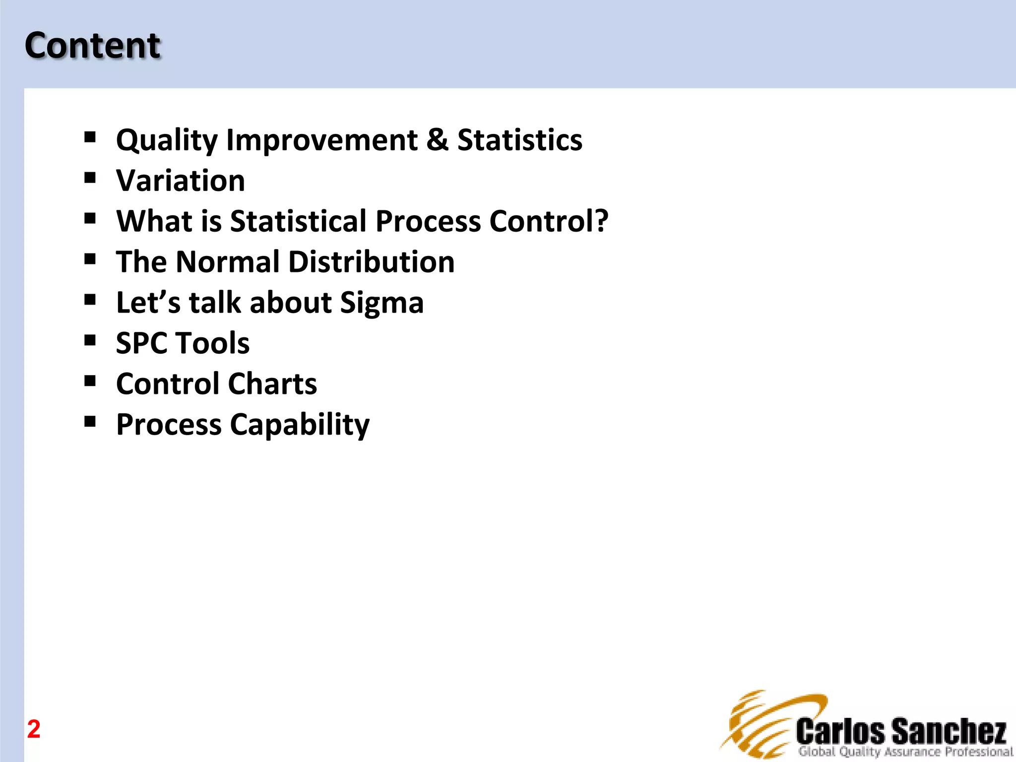
Introduction to Statistical Process Control with key topics like Quality Improvement, Variation, SPC tools including Control Charts and Process Capability.
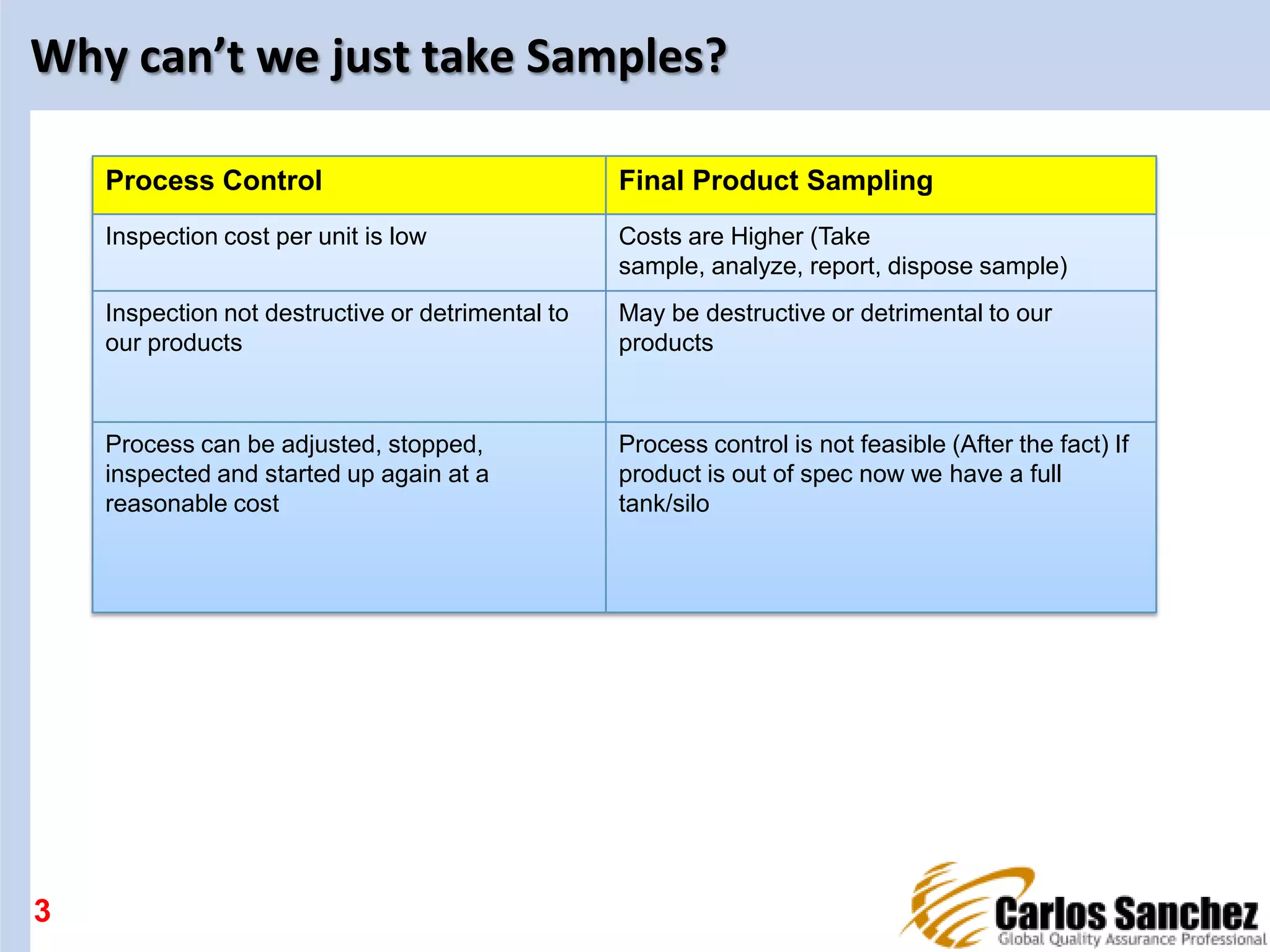
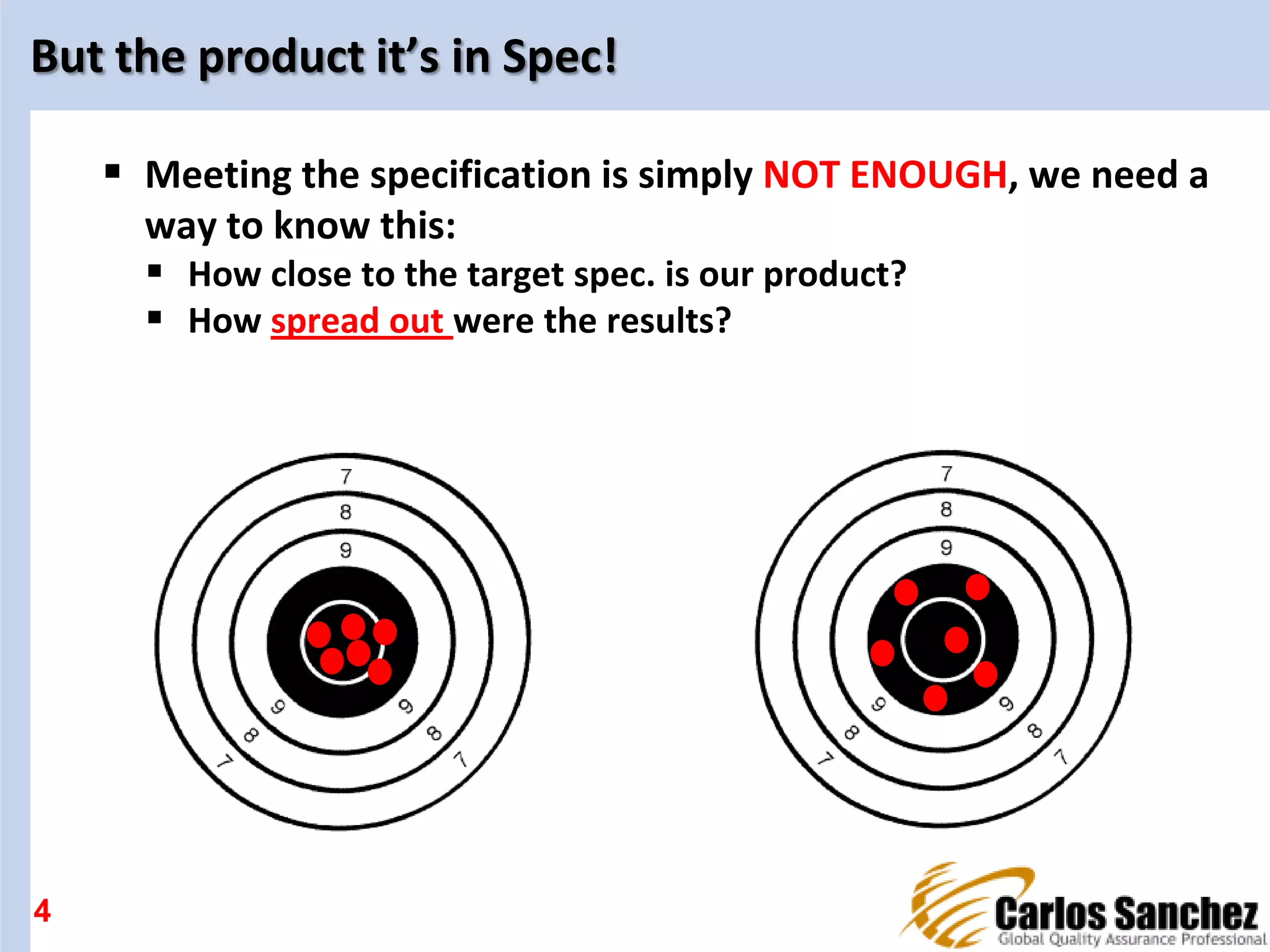
Explains the limitations of sampling in process control and emphasizes the need to assess how products meet specifications.
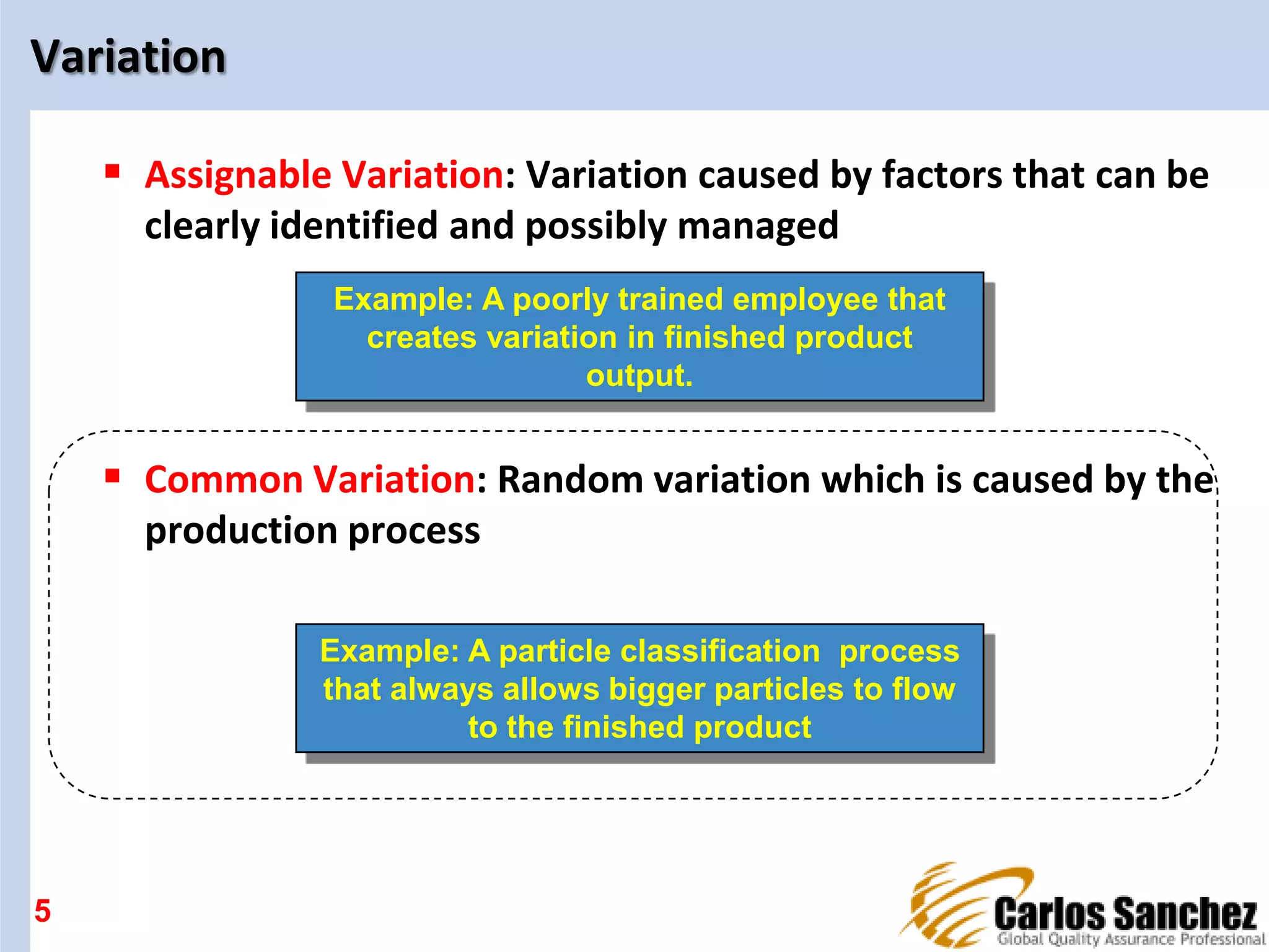
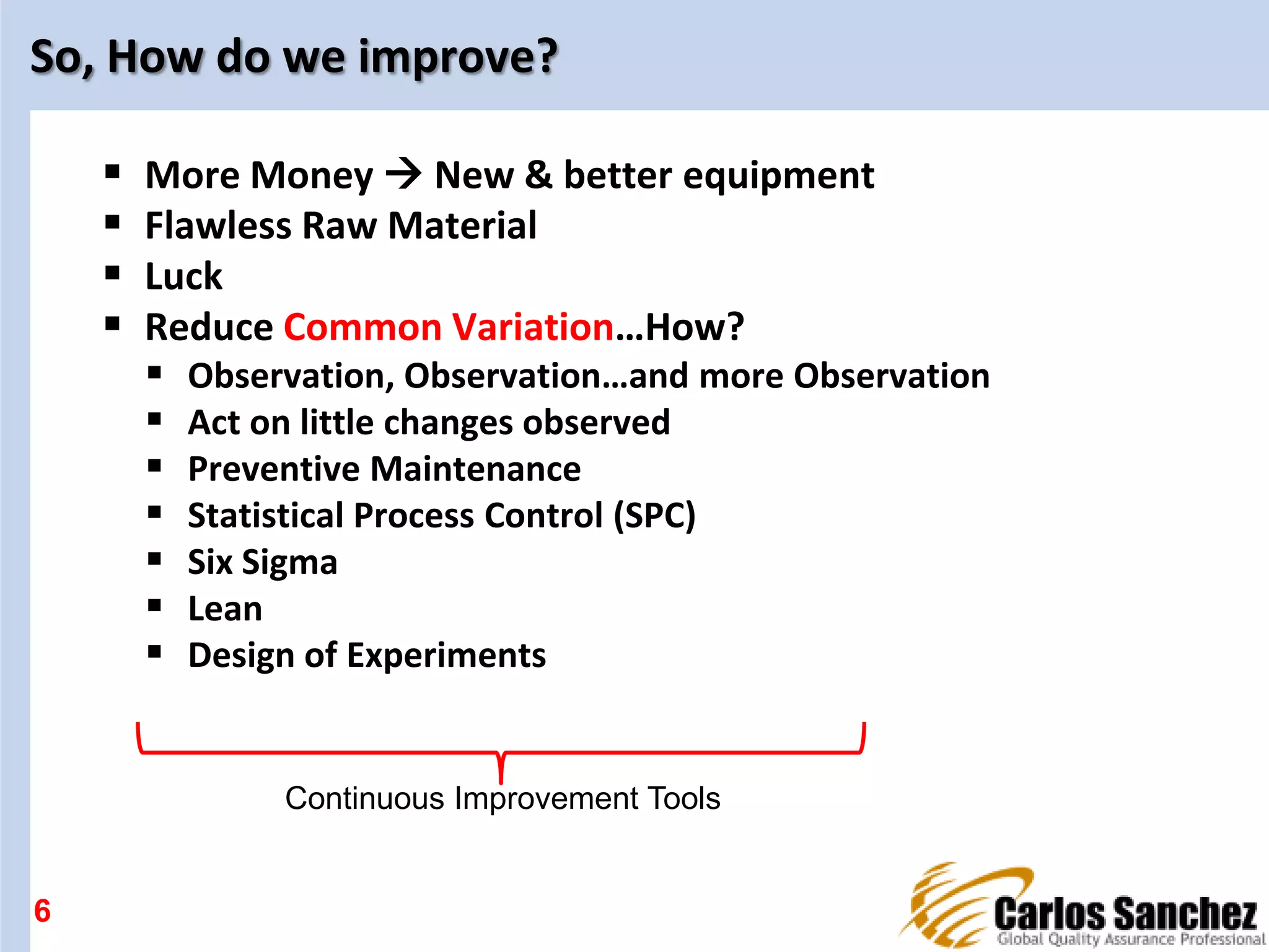
Details on assignable and common variation, ways to improve process control like SPC, Six Sigma, and Lean methods.
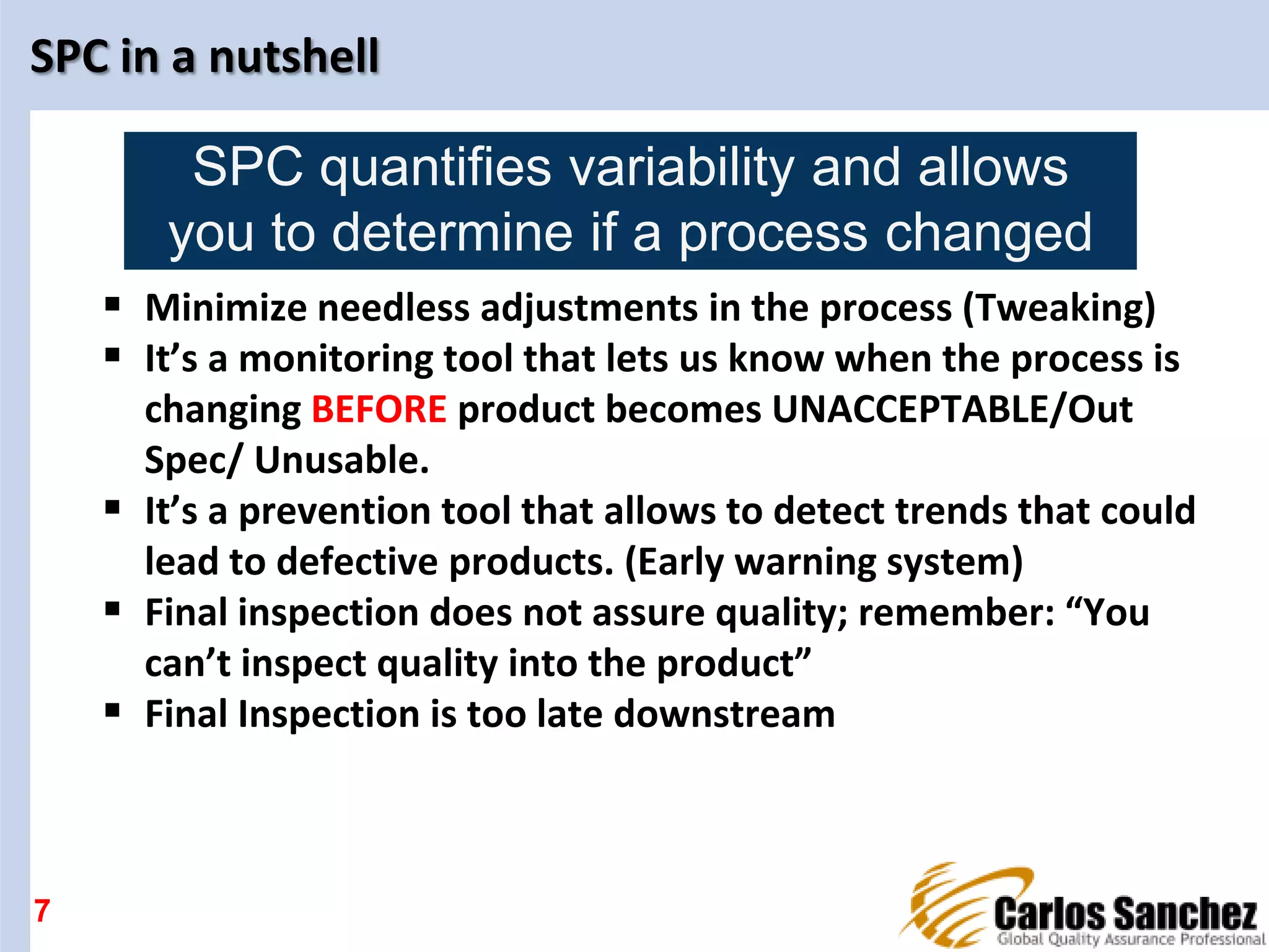
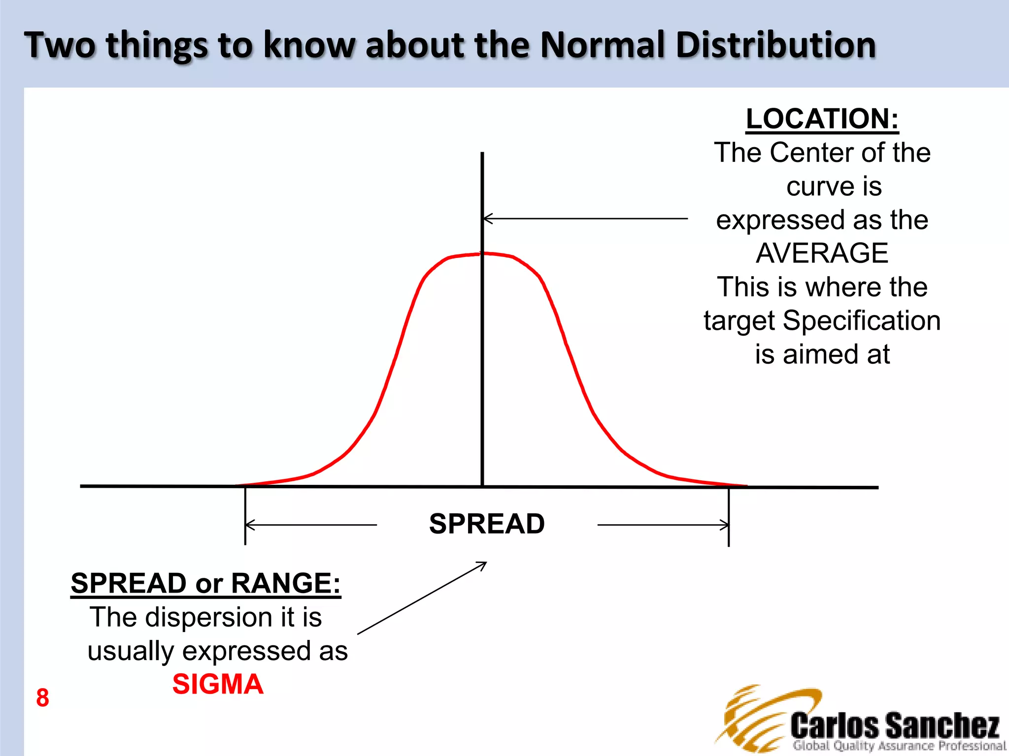
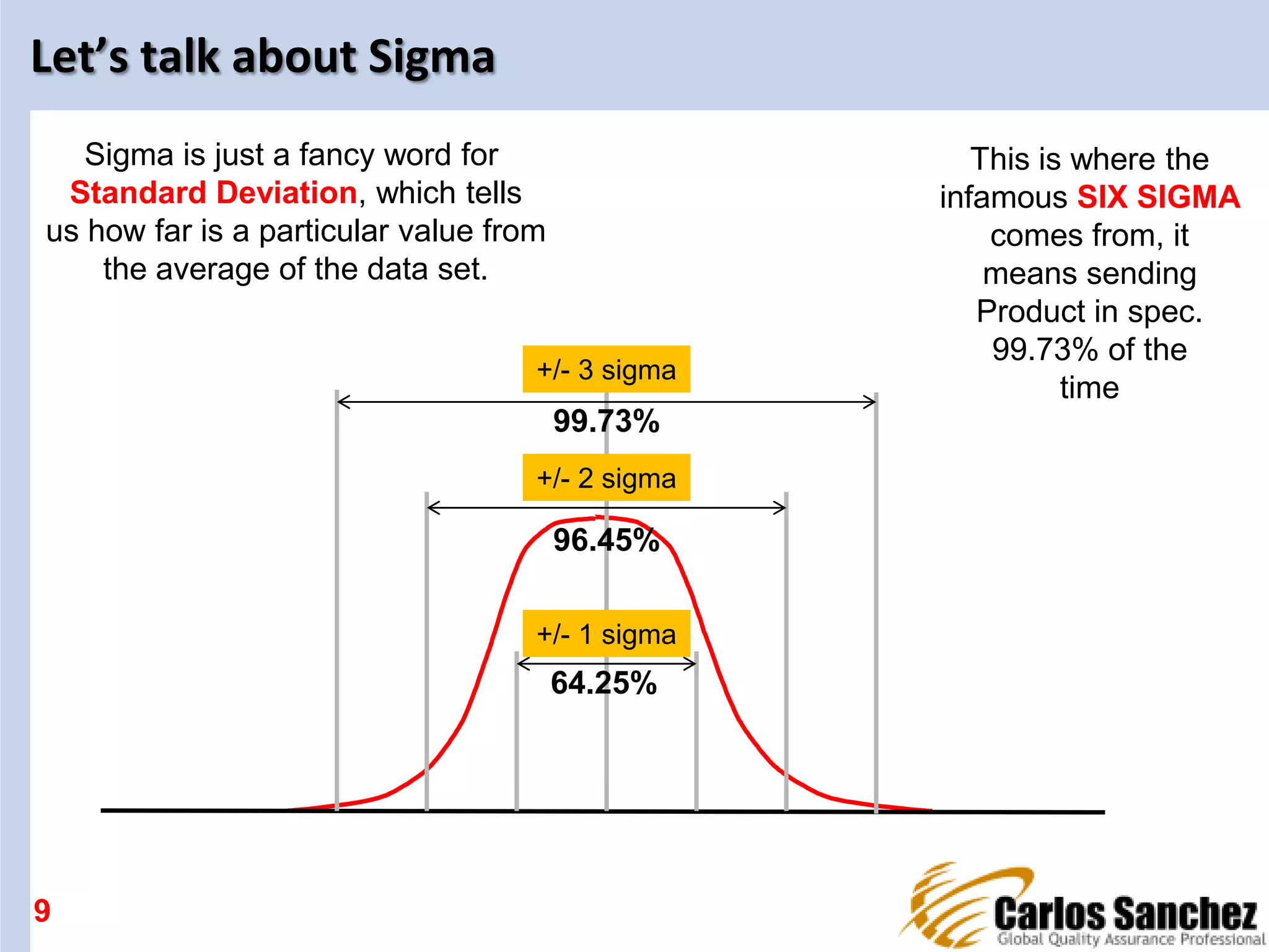
SPC as a tool to monitor process changes and its relation to the Normal Distribution and Sigma (standard deviation).
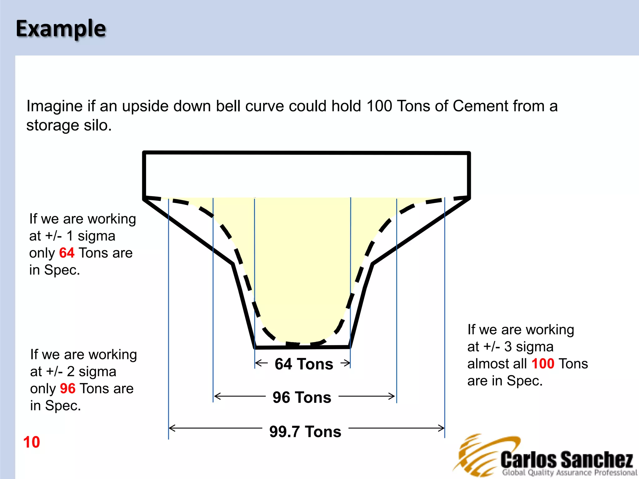
Illustration of how different sigma levels (1, 2, 3) impact product specification compliance.
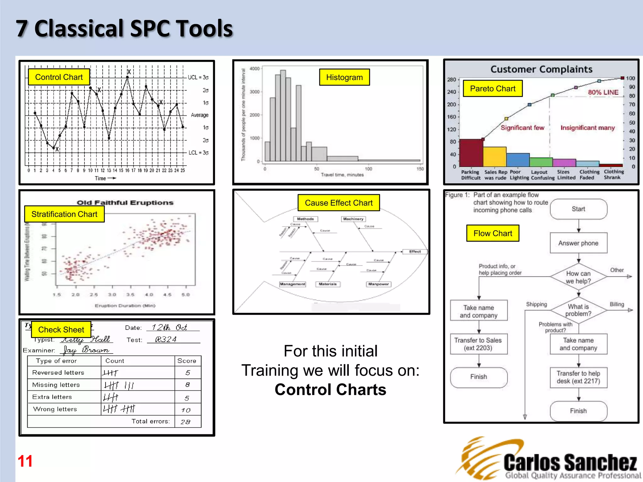
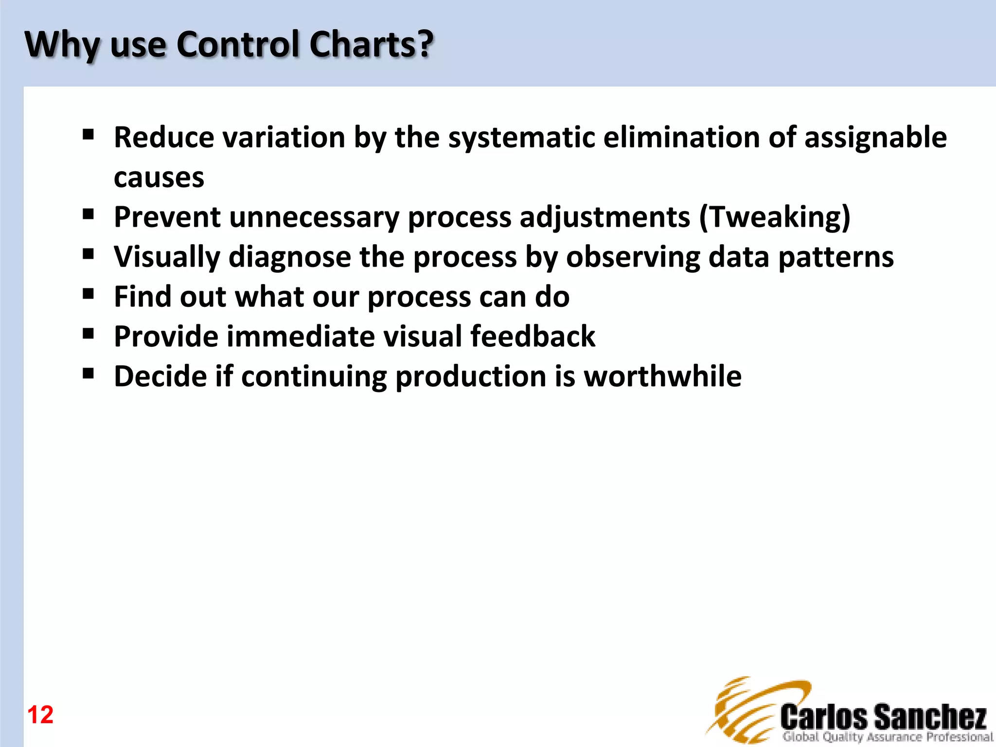
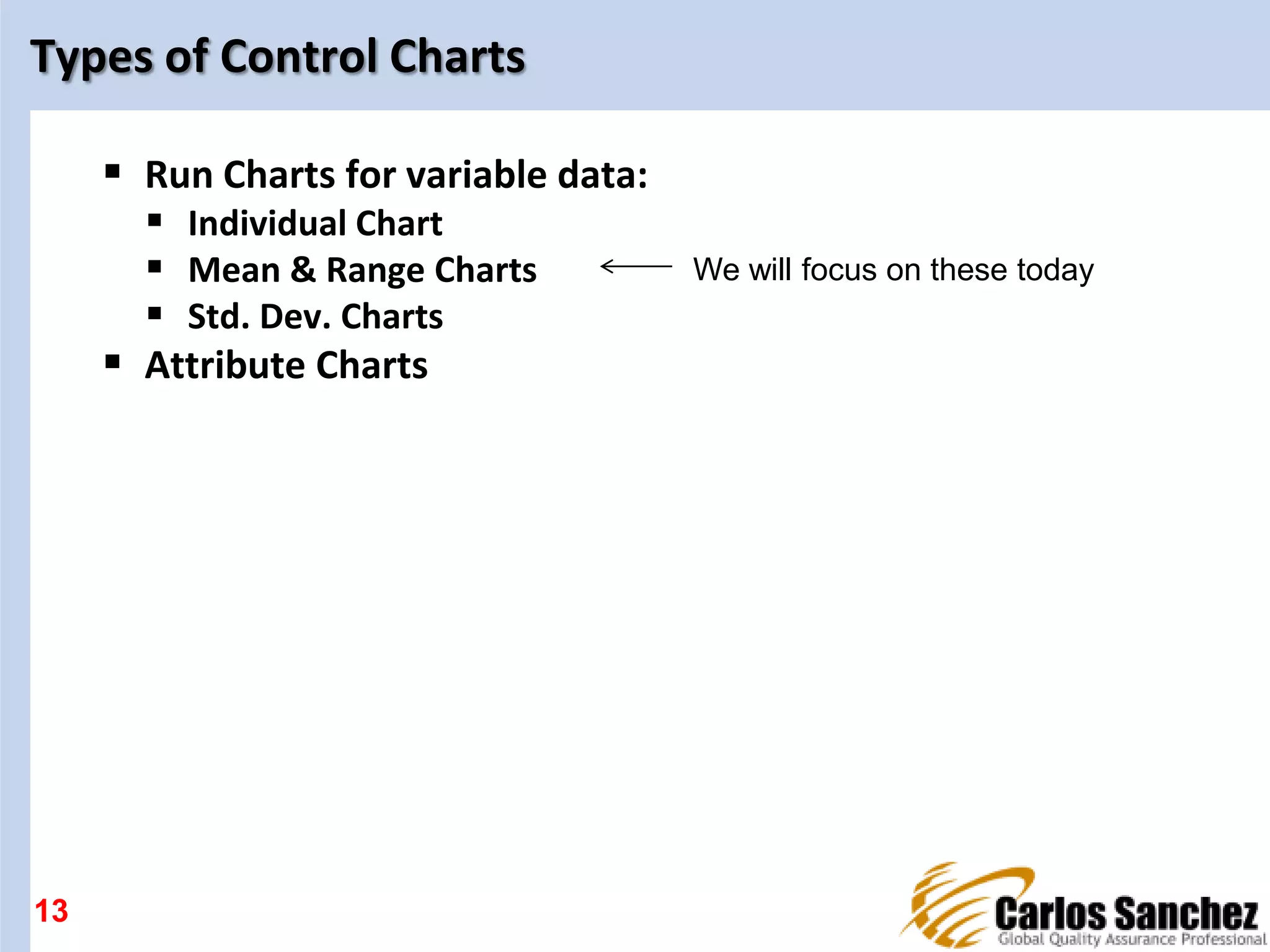
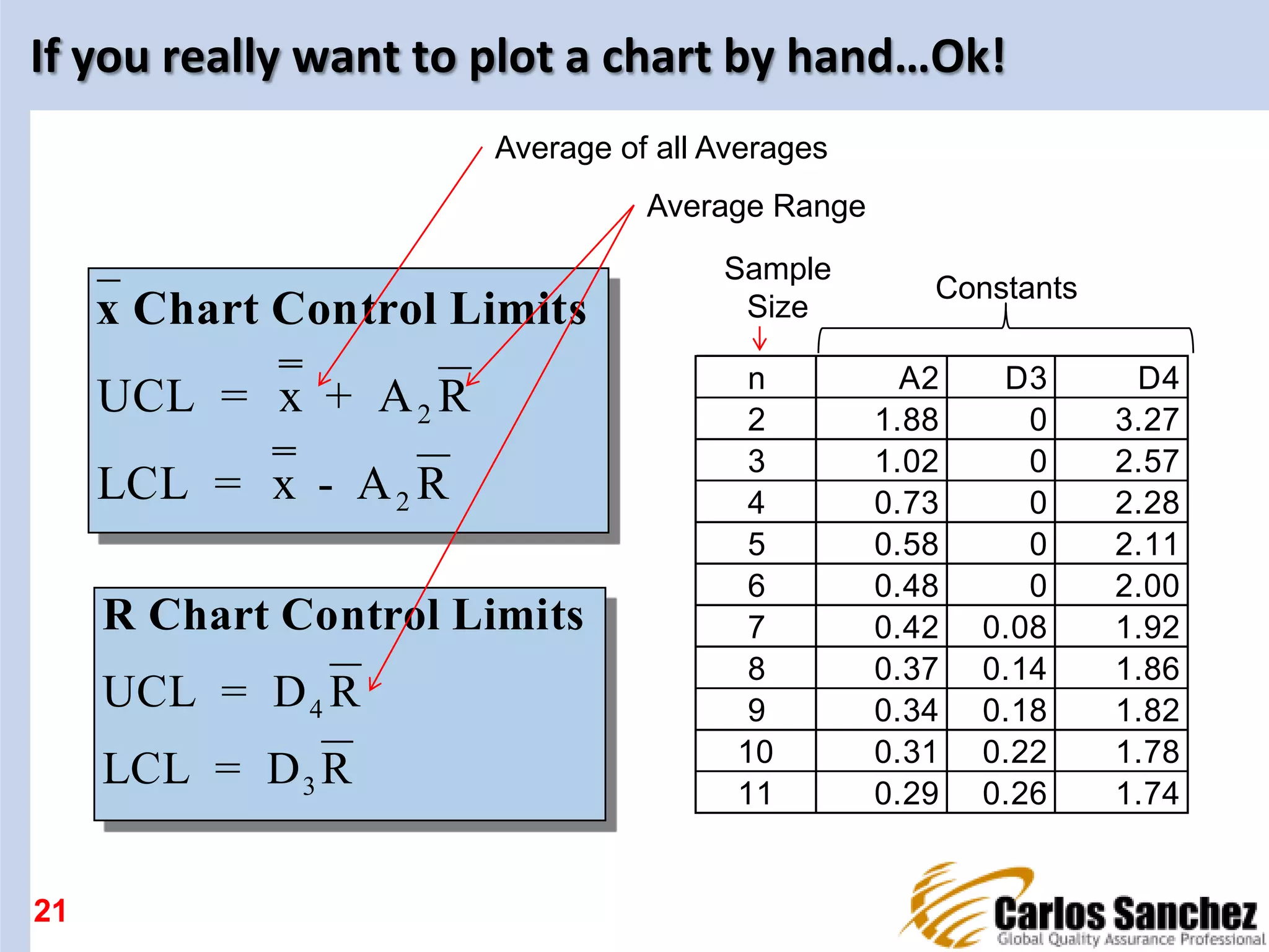
Introduction to classical SPC tools, focusing on the use of Control Charts for process analysis.
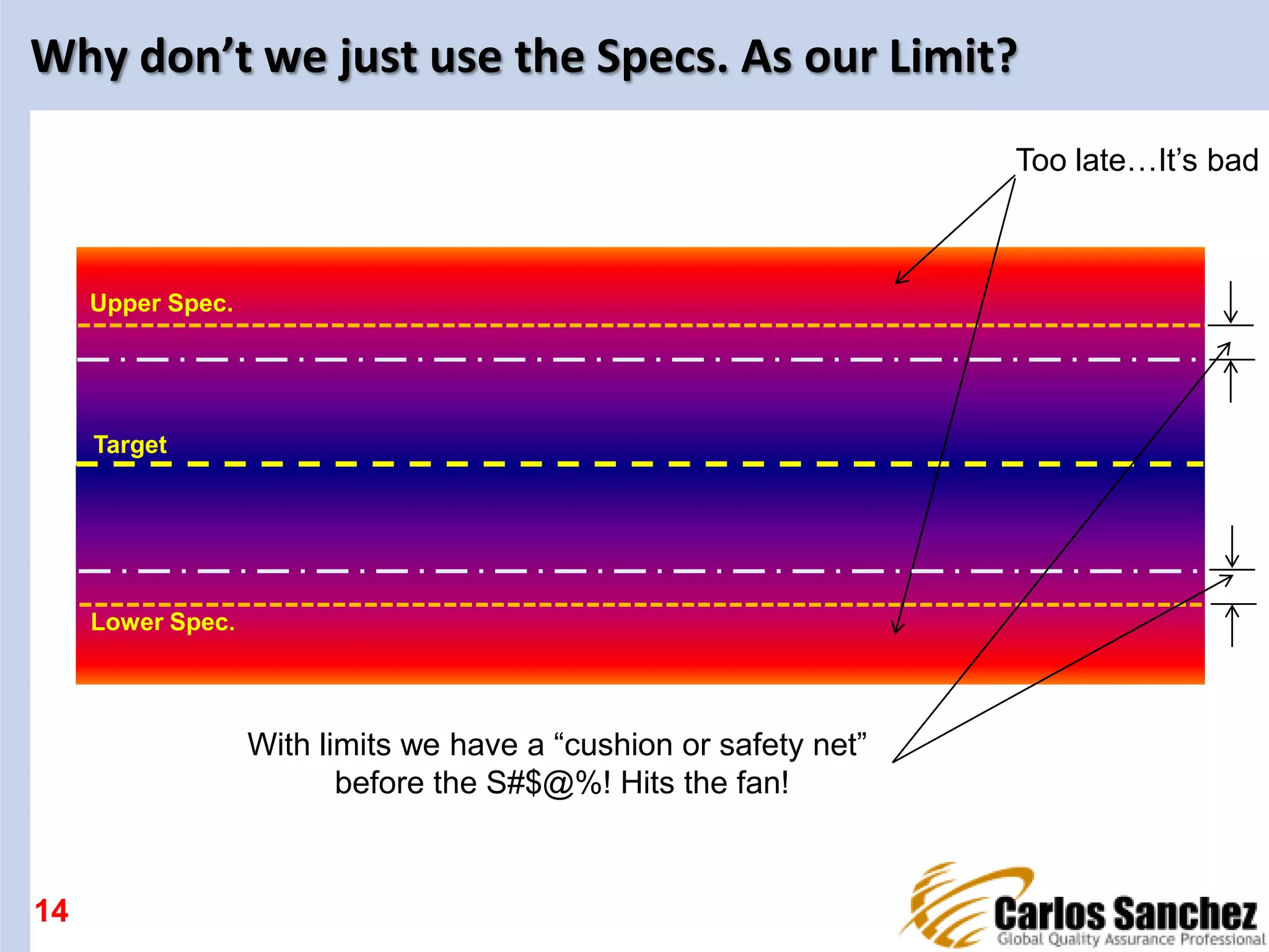
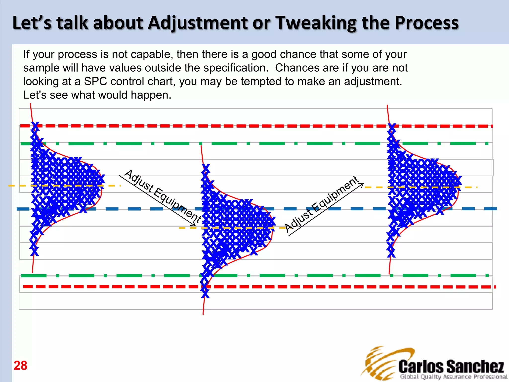
Justification for using control limits in monitoring processes instead of merely relying on specifications.
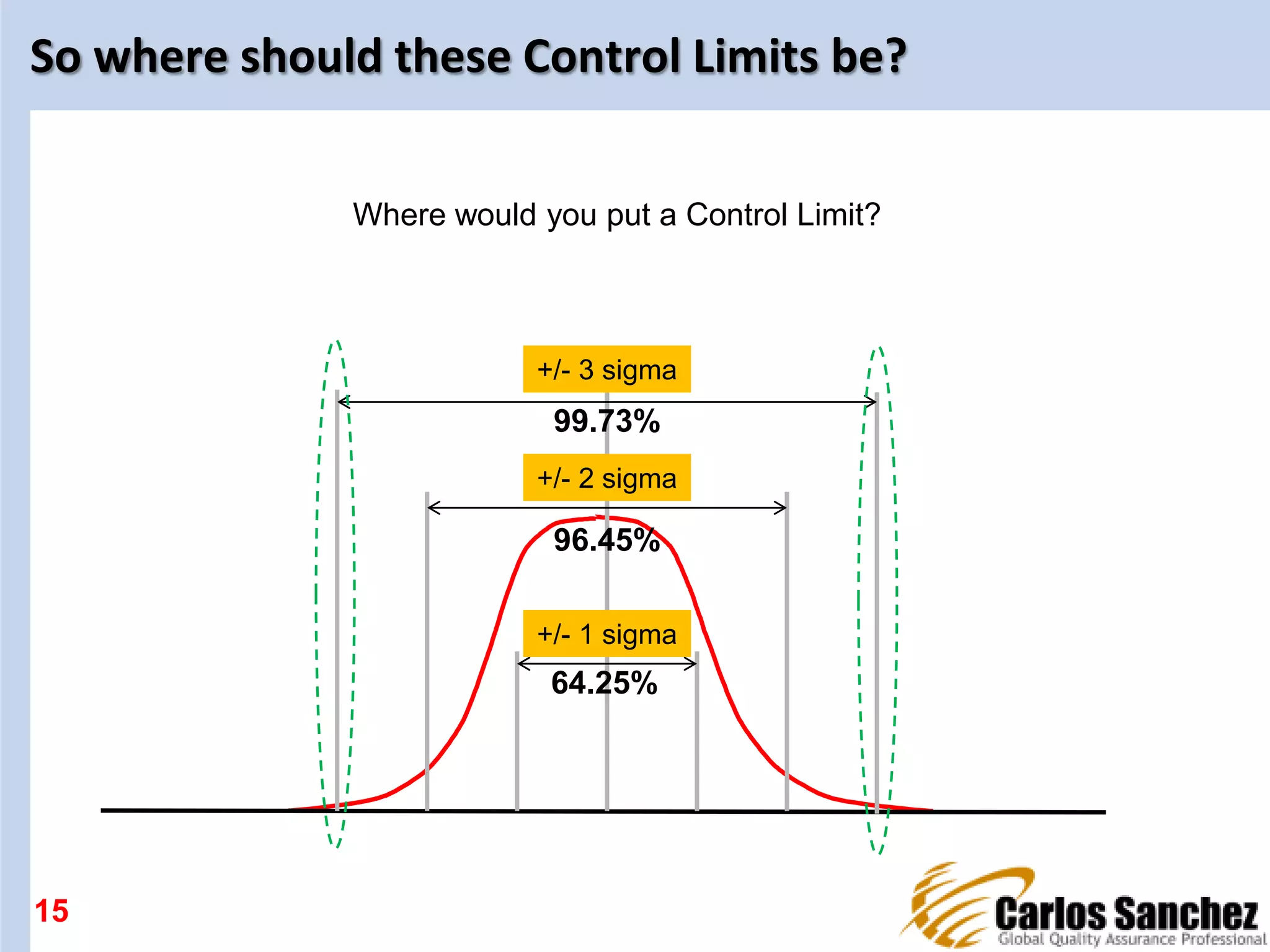
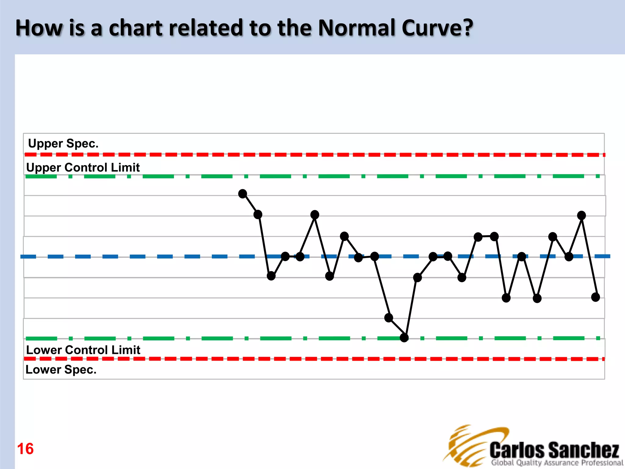
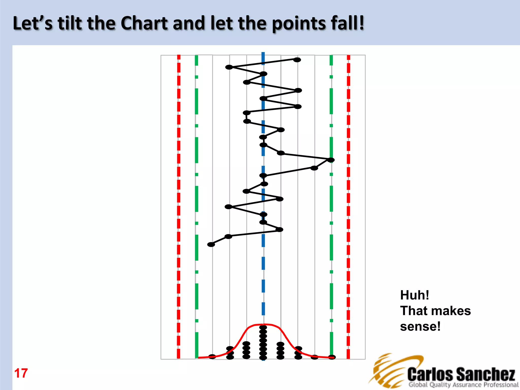
Understanding how control limits relate to the Normal Curve and central tendency in data analysis.
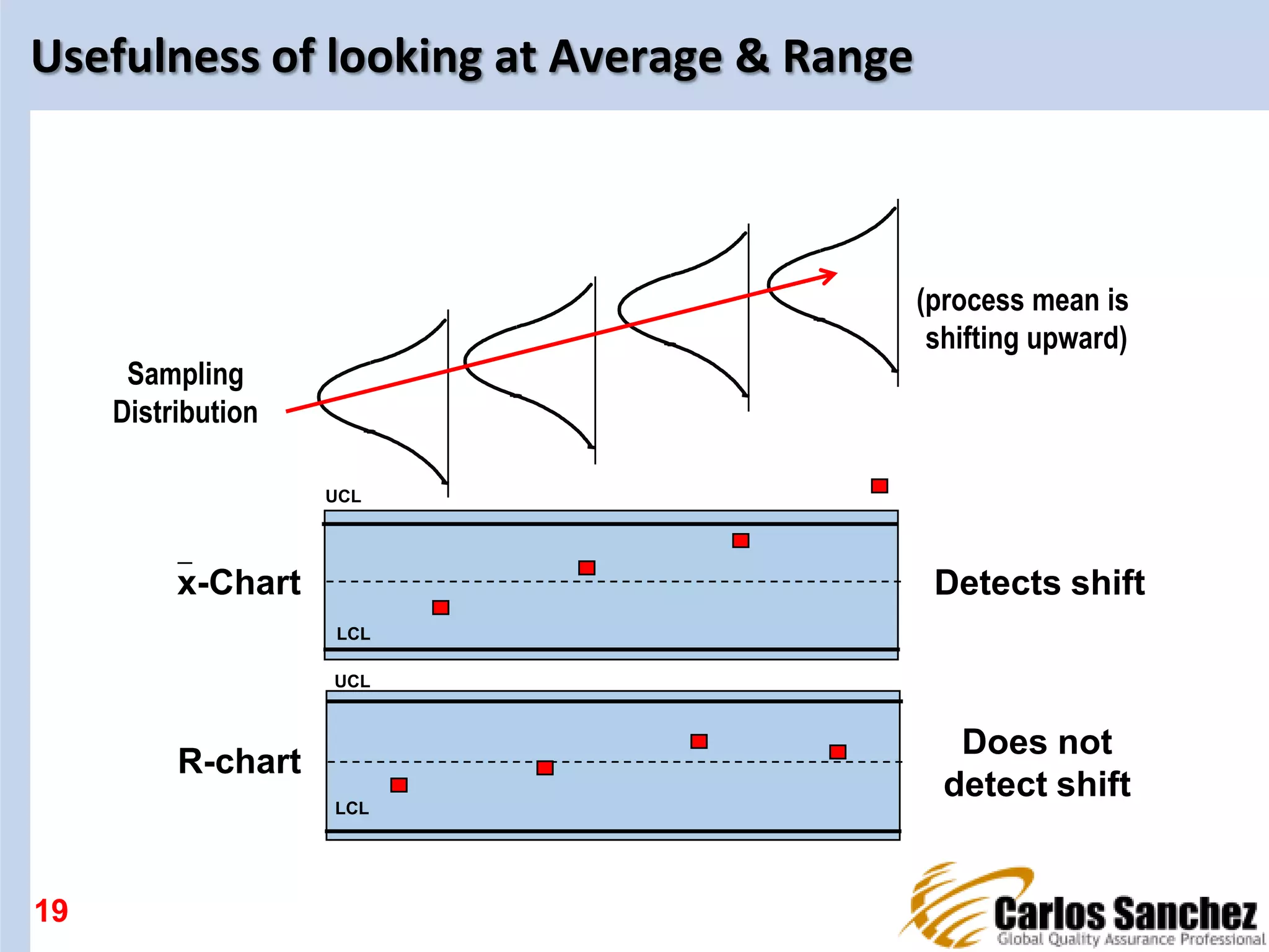
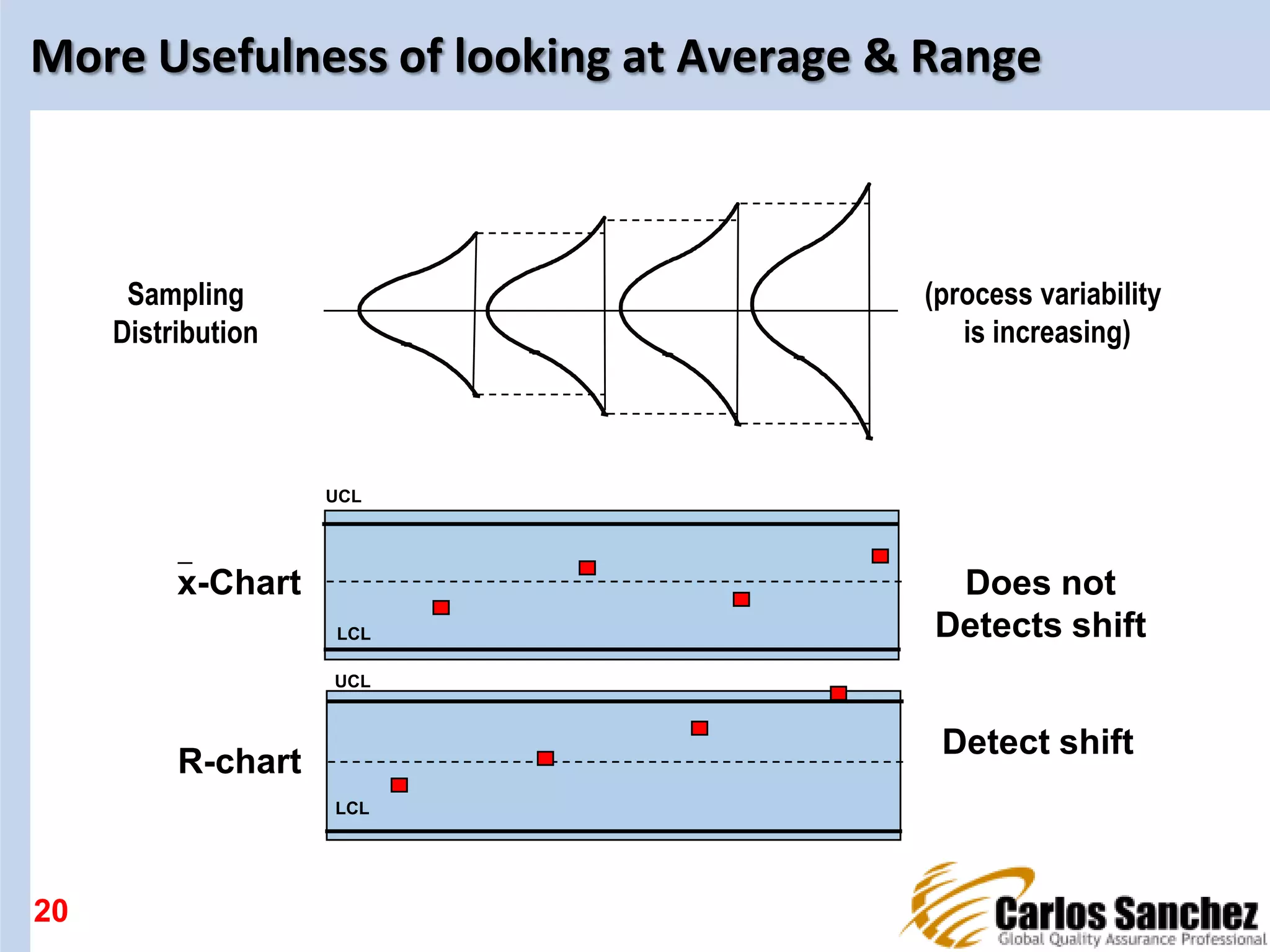
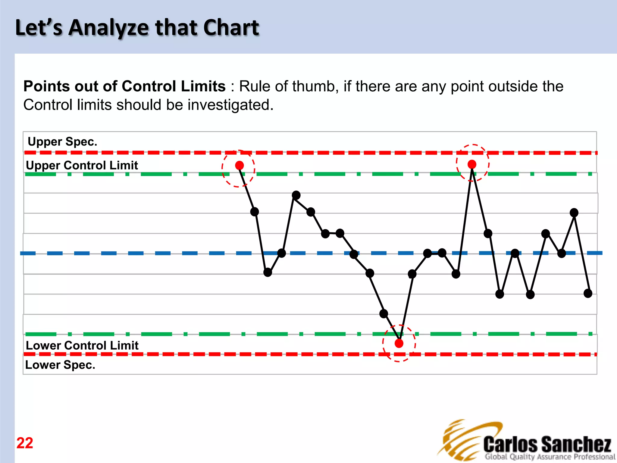
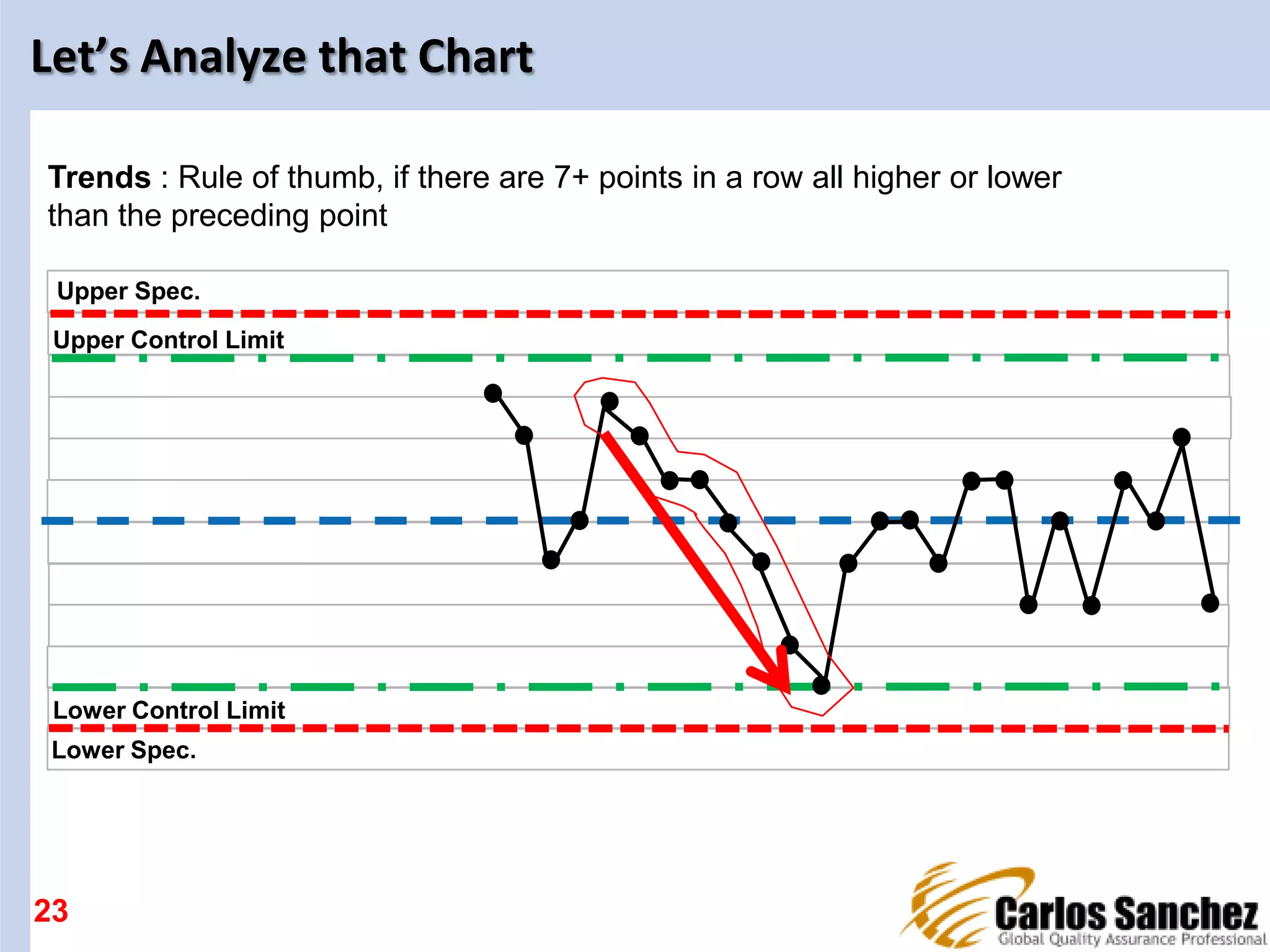
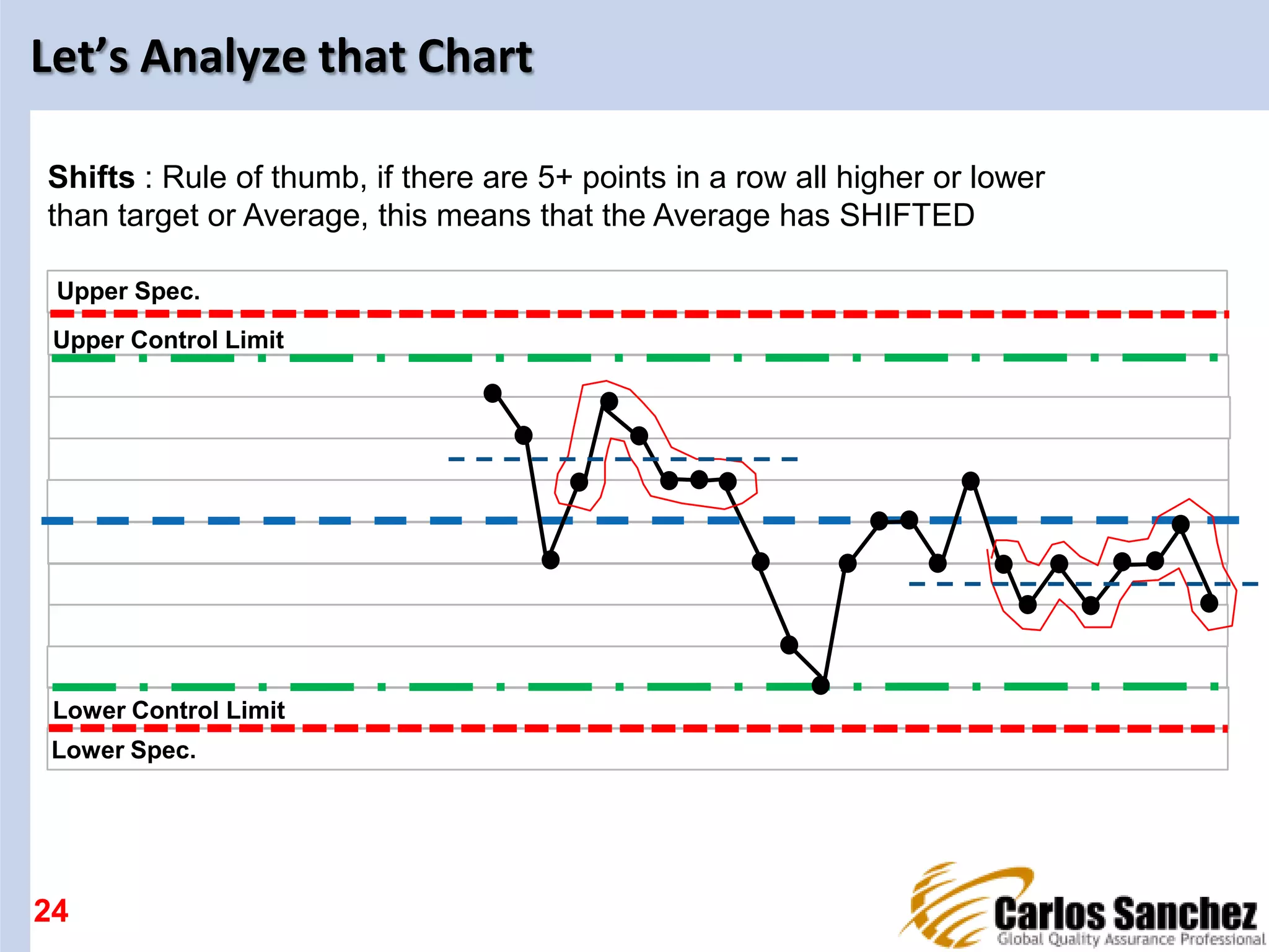
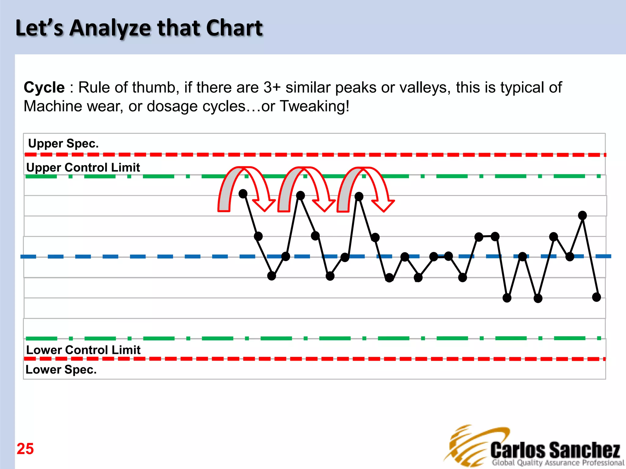
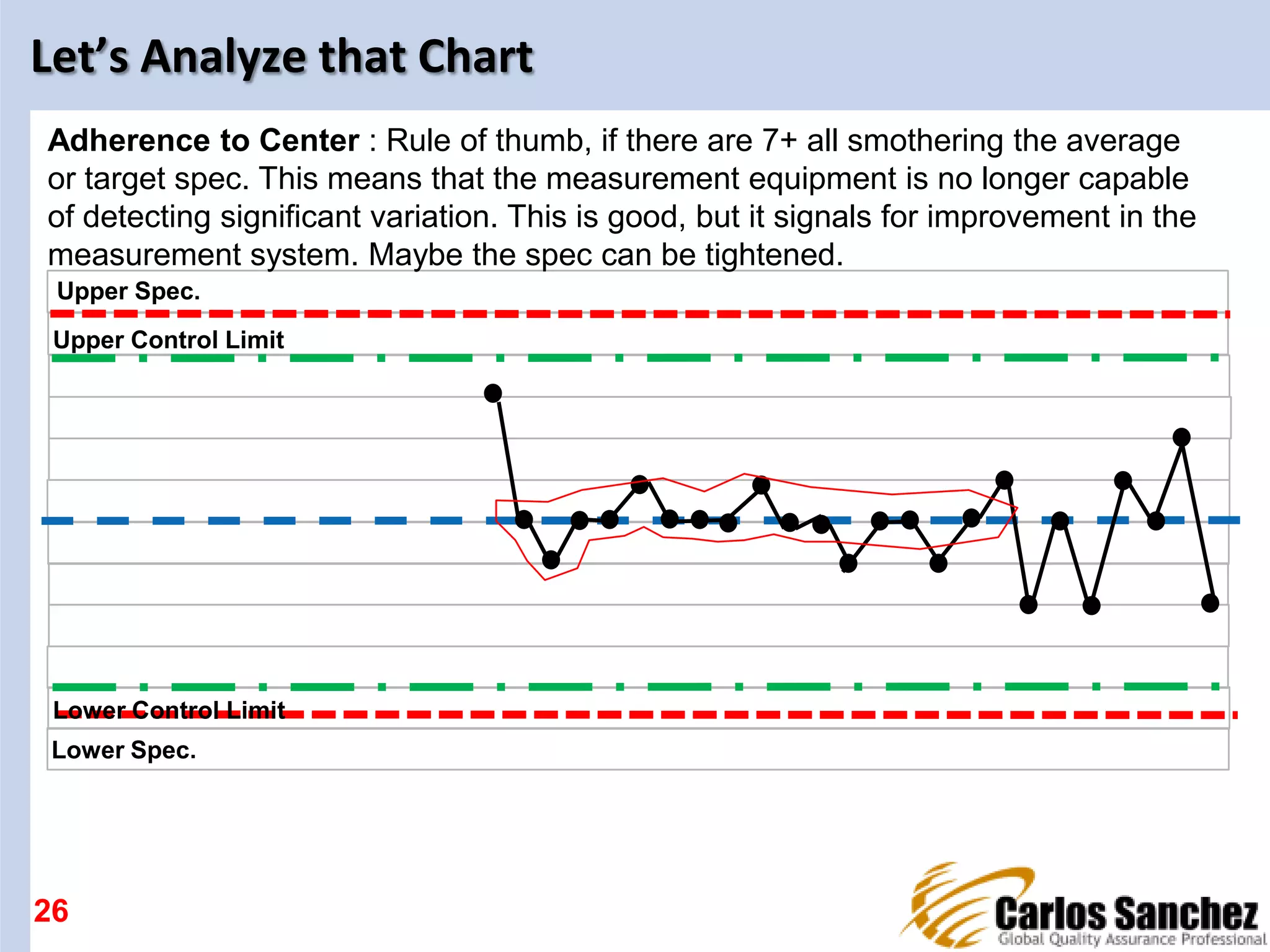
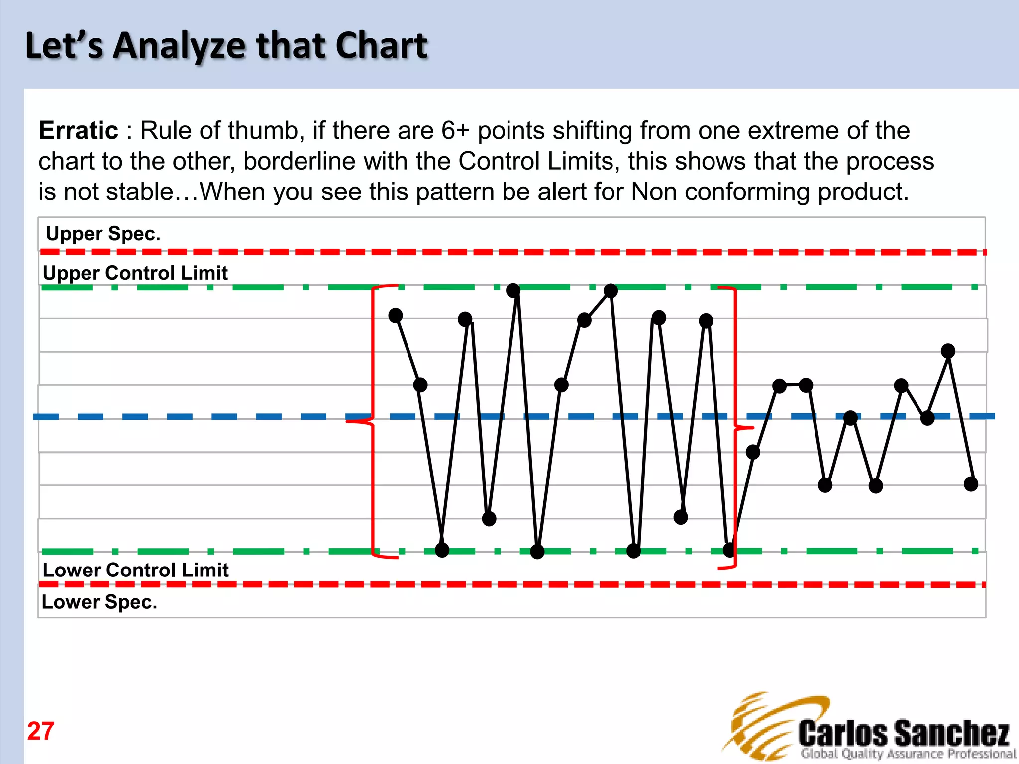
Analyzing control charts to detect shifts, trends, and the significance of measurement stability.
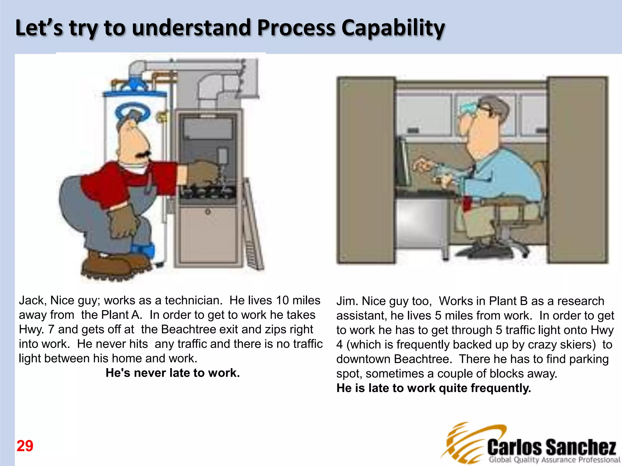
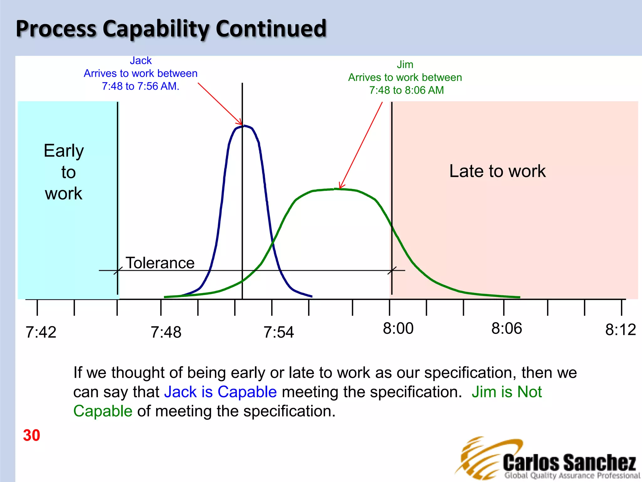
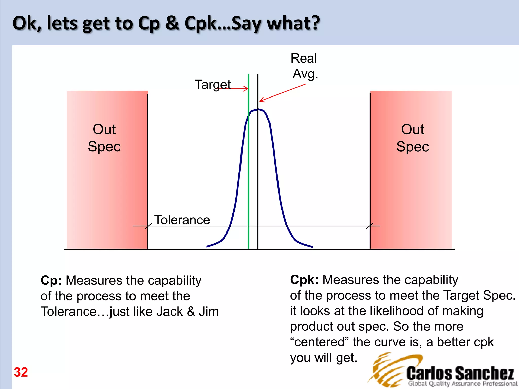
Illustrative examples to explain process capability with respect to meeting specifications in practical scenarios.
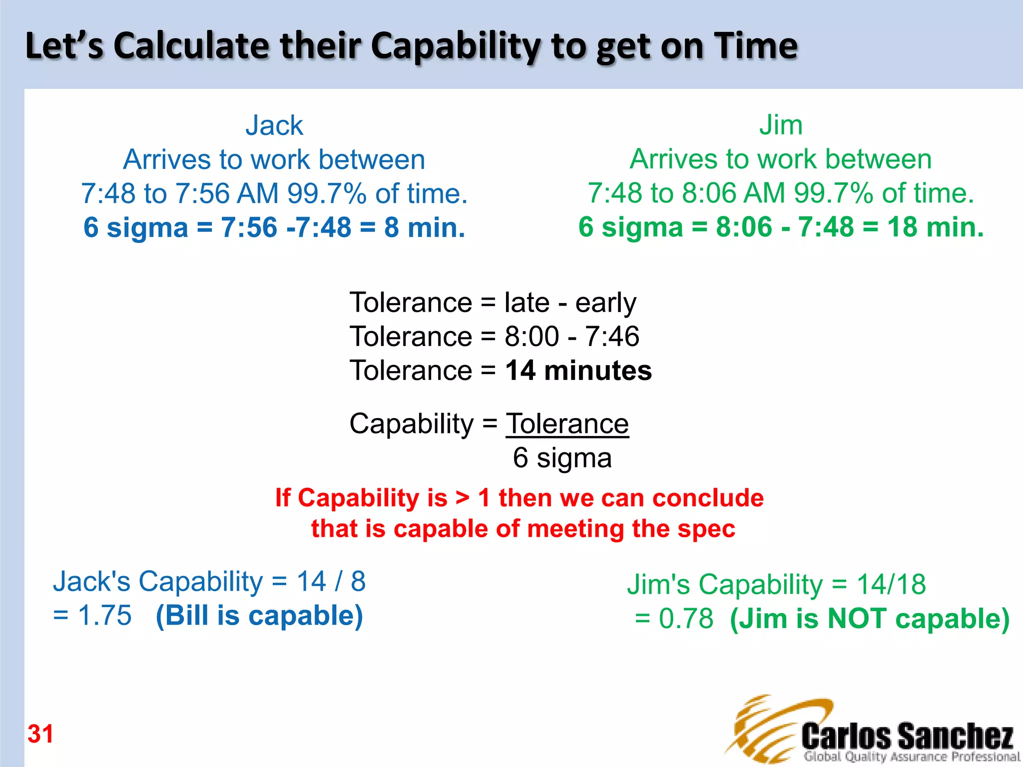
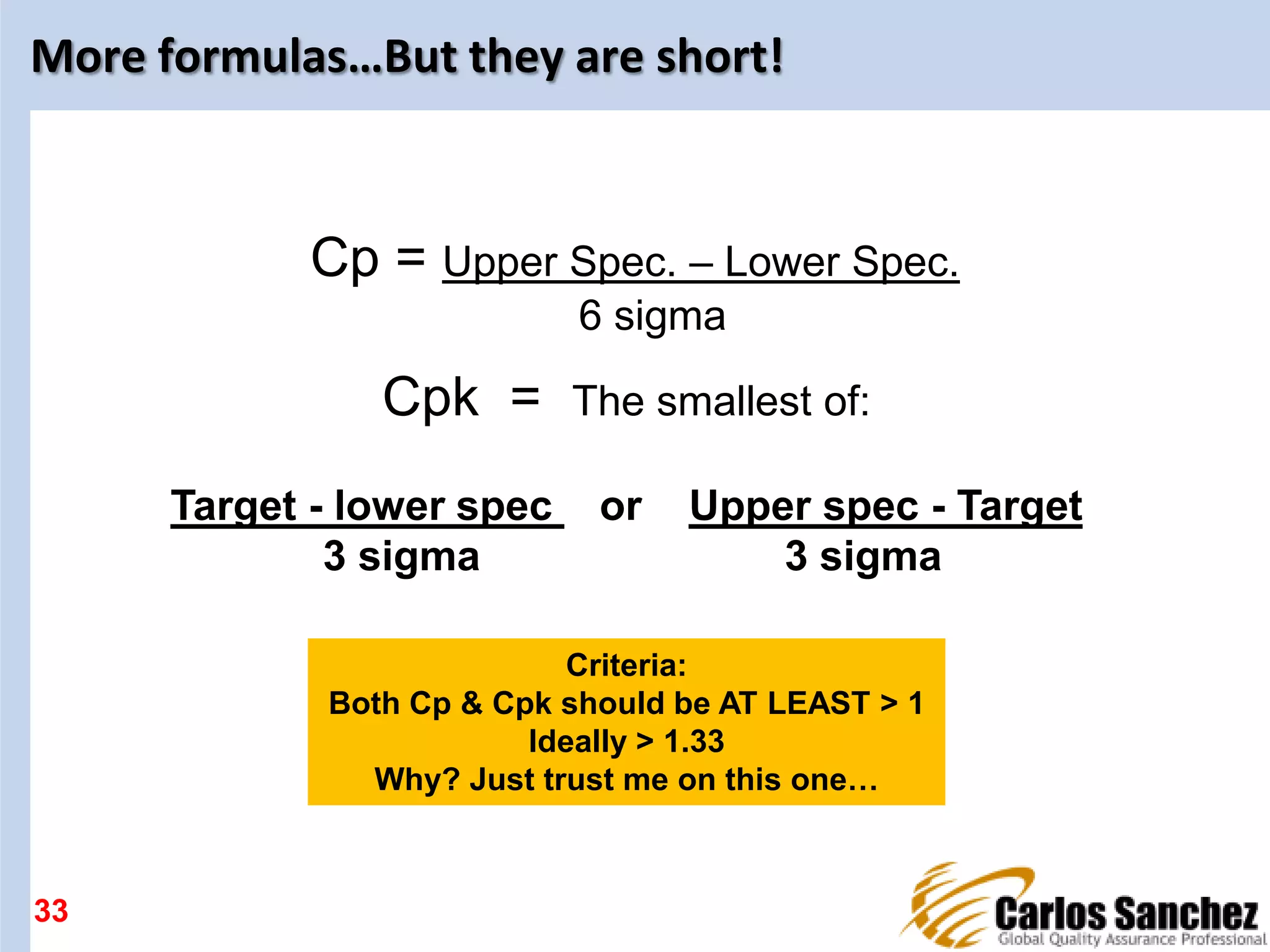
Introduction to process capability indices Cp and Cpk, emphasizing their importance in evaluating process performance.
2
Content
Quality Improvement& Statistics
Variation
What is Statistical Process Control?
The Normal Distribution
Let’s talk about Sigma
SPC Tools
Control Charts
Process Capability
3.
Why can’t wejust take Samples?
3
Process Control Final Product Sampling
Inspection cost per unit is low Costs are Higher (Take
sample, analyze, report, dispose sample)
Inspection not destructive or detrimental to
our products
May be destructive or detrimental to our
products
Process can be adjusted, stopped,
inspected and started up again at a
reasonable cost
Process control is not feasible (After the fact) If
product is out of spec now we have a full
tank/silo
4.
But the productit’s in Spec!
Meeting the specification is simply NOT ENOUGH, we need a
way to know this:
How close to the target spec. is our product?
How spread out were the results?
4
5.
Variation
Assignable Variation:Variation caused by factors that can be
clearly identified and possibly managed
Common Variation: Random variation which is caused by the
production process
5
Example: A poorly trained employee that
creates variation in finished product
output.
Example: A particle classification process
that always allows bigger particles to flow
to the finished product
6.
So, How dowe improve?
More Money New & better equipment
Flawless Raw Material
Luck
Reduce Common Variation…How?
Observation, Observation…and more Observation
Act on little changes observed
Preventive Maintenance
Statistical Process Control (SPC)
Six Sigma
Lean
Design of Experiments
6
Continuous Improvement Tools
7.
SPC in anutshell
Minimize needless adjustments in the process (Tweaking)
It’s a monitoring tool that lets us know when the process is
changing BEFORE product becomes UNACCEPTABLE/Out
Spec/ Unusable.
It’s a prevention tool that allows to detect trends that could
lead to defective products. (Early warning system)
Final inspection does not assure quality; remember: “You
can’t inspect quality into the product”
Final Inspection is too late downstream
7
SPC quantifies variability and allows
you to determine if a process changed
8.
Two things toknow about the Normal Distribution
SPREAD
LOCATION:
The Center of the
curve is
expressed as the
AVERAGE
This is where the
target Specification
is aimed at
SPREAD or RANGE:
The dispersion it is
usually expressed as
SIGMA8
9.
Let’s talk aboutSigma
9
Sigma is just a fancy word for
Standard Deviation, which tells
us how far is a particular value from
the average of the data set.
+/- 1 sigma
+/- 2 sigma
+/- 3 sigma
64.25%
96.45%
99.73%
This is where the
infamous SIX SIGMA
comes from, it
means sending
Product in spec.
99.73% of the
time
10.
Example
64 Tons
96 Tons
99.7Tons
Imagine if an upside down bell curve could hold 100 Tons of Cement from a
storage silo.
If we are working
at +/- 1 sigma
only 64 Tons are
in Spec.
If we are working
at +/- 2 sigma
only 96 Tons are
in Spec.
If we are working
at +/- 3 sigma
almost all 100 Tons
are in Spec.
10
11.
7 Classical SPCTools
11
Histogram
Pareto Chart
Control Chart
Stratification Chart
Cause Effect Chart
Flow Chart
Check Sheet
For this initial
Training we will focus on:
Control Charts
12.
Why use ControlCharts?
Reduce variation by the systematic elimination of assignable
causes
Prevent unnecessary process adjustments (Tweaking)
Visually diagnose the process by observing data patterns
Find out what our process can do
Provide immediate visual feedback
Decide if continuing production is worthwhile
12
13.
Types of ControlCharts
Run Charts for variable data:
Individual Chart
Mean & Range Charts
Std. Dev. Charts
Attribute Charts
13
We will focus on these today
14.
Why don’t wejust use the Specs. As our Limit?
14
Too late…It’s bad
Upper Spec.
Lower Spec.
Target
With limits we have a “cushion or safety net”
before the S#$@%! Hits the fan!
15.
So where shouldthese Control Limits be?
15
+/- 1 sigma
+/- 2 sigma
+/- 3 sigma
64.25%
96.45%
99.73%
Where would you put a Control Limit?
16.
How is achart related to the Normal Curve?
16
Upper Spec.
Lower Spec.
Upper Control Limit
Lower Control Limit
17.
Let’s tilt theChart and let the points fall!
17
Huh!
That makes
sense!
18.
At the endit averages out!
When the population is big, looking at individuals to detect
trends is tricky…
It’s been proven that when you look at averages these tend
to behave like a Normal Curve
Google this: Central Limit Theorem (It’s great for those sleepless nights)
So from now on this training all example charts are based on
Averages. This means that a “Point” in a control charts
represents the “Average” value of a sample (Typical sample
size varies from 3 to 5), I like 5, but heck, you can choose
whatever size you want
18
19.
Usefulness of lookingat Average & Range
19
UCL
LCL
UCL
LCL
R-chart
x-Chart Detects shift
Does not
detect shift
(process mean is
shifting upward)
Sampling
Distribution
20.
More Usefulness oflooking at Average & Range
20
UCL
LCL
UCL
LCL
R-chart
x-Chart Does not
Detects shift
Detect shift
(process variability
is increasing)
Sampling
Distribution
21.
If you reallywant to plot a chart by hand…Ok!
21
x Chart Control Limits
UCL = x + A R
LCL = x - A R
2
2
R Chart Control Limits
UCL = D R
LCL = D R
4
3
n A2 D3 D4
2 1.88 0 3.27
3 1.02 0 2.57
4 0.73 0 2.28
5 0.58 0 2.11
6 0.48 0 2.00
7 0.42 0.08 1.92
8 0.37 0.14 1.86
9 0.34 0.18 1.82
10 0.31 0.22 1.78
11 0.29 0.26 1.74
Average of all Averages
Average Range
Constants
Sample
Size
22.
Let’s Analyze thatChart
22
Upper Spec.
Lower Spec.
Upper Control Limit
Lower Control Limit
Points out of Control Limits : Rule of thumb, if there are any point outside the
Control limits should be investigated.
23.
Let’s Analyze thatChart
23
Upper Spec.
Lower Spec.
Upper Control Limit
Lower Control Limit
Trends : Rule of thumb, if there are 7+ points in a row all higher or lower
than the preceding point
24.
Let’s Analyze thatChart
24
Upper Spec.
Lower Spec.
Upper Control Limit
Lower Control Limit
Shifts : Rule of thumb, if there are 5+ points in a row all higher or lower
than target or Average, this means that the Average has SHIFTED
25.
Let’s Analyze thatChart
25
Upper Spec.
Lower Spec.
Upper Control Limit
Lower Control Limit
Cycle : Rule of thumb, if there are 3+ similar peaks or valleys, this is typical of
Machine wear, or dosage cycles…or Tweaking!
26.
Let’s Analyze thatChart
26
Upper Spec.
Lower Spec.
Upper Control Limit
Lower Control Limit
Adherence to Center : Rule of thumb, if there are 7+ all smothering the average
or target spec. This means that the measurement equipment is no longer capable
of detecting significant variation. This is good, but it signals for improvement in the
measurement system. Maybe the spec can be tightened.
27.
Let’s Analyze thatChart
27
Upper Spec.
Lower Spec.
Upper Control Limit
Lower Control Limit
Erratic : Rule of thumb, if there are 6+ points shifting from one extreme of the
chart to the other, borderline with the Control Limits, this shows that the process
is not stable…When you see this pattern be alert for Non conforming product.
28.
Let’s talk aboutAdjustment or Tweaking the Process
28
x
xx
xxxxxxx
xx
x
xx
xxxxxxx
xxx
x
xxxxxxx
xxx
x
xxxxxxx
x
x
x
xxx
x
xxx
xxxxxx
xx
x
xxxxx x
xxxxxxxxxxxxxxxxxxxxxxxxxxxxxxxxxx
xx x
xxx
xxxx
x
xxx
x
xxxxxxxx
xxxxxxxx
x
x
x
x x
x
xx
x
x
If your process is not capable, then there is a good chance that some of your
sample will have values outside the specification. Chances are if you are not
looking at a SPC control chart, you may be tempted to make an adjustment.
Let's see what would happen.
x
xx
xxxxxxx
xx
x
xx
xxxxxxx
xxx
x
xxxxxxx
xxx
x
xxxxxxx
x
x
x
xxx
x
xxx
xxxxxx
xx
x
xxxxx x
xxxxxxxxxxxxxxxxxxxxxxxxxxxxxxxxxx
xx x
xxx
xxxx
x
xxx
x
xxxxxxxx
xxxxxxxx
x
x
x
x x
x
xx
x
x
x
xx
xxxxxxx
xx
x
xx
xxxxxxx
xxx
x
xxxxxxx
xxx
x
xxxxxxx
x
x
x
xxx
x
xxx
xxxxxx
xx
x
xxxxx x
xxxxxxxxxxxxxxxxxxxxxxxxxxxxxxxxxx
xx x
xxx
xxxx
x
xxx
x
xxxxxxxx
xxxxxxxx
x
x
x
x x
x
xx
x
x
29.
Let’s try tounderstand Process Capability
29
Jim. Nice guy too, Works in Plant B as a research
assistant, he lives 5 miles from work. In order to get
to work he has to get through 5 traffic light onto Hwy
4 (which is frequently backed up by crazy skiers) to
downtown Beachtree. There he has to find parking
spot, sometimes a couple of blocks away.
He is late to work quite frequently.
Jack, Nice guy; works as a technician. He lives 10 miles
away from the Plant A. In order to get to work he takes
Hwy. 7 and gets off at the Beachtree exit and zips right
into work. He never hits any traffic and there is no traffic
light between his home and work.
He's never late to work.
30.
Process Capability Continued
30
8:068:128:007:547:487:42
Late to work
Early
to
work
Jack
Arrives to work between
7:48 to 7:56 AM.
Jim
Arrives to work between
7:48 to 8:06 AM
If we thought of being early or late to work as our specification, then we
can say that Jack is Capable meeting the specification. Jim is Not
Capable of meeting the specification.
Tolerance
31.
Let’s Calculate theirCapability to get on Time
31
Jack
Arrives to work between
7:48 to 7:56 AM 99.7% of time.
6 sigma = 7:56 -7:48 = 8 min.
Jim
Arrives to work between
7:48 to 8:06 AM 99.7% of time.
6 sigma = 8:06 - 7:48 = 18 min.
Tolerance = late - early
Tolerance = 8:00 - 7:46
Tolerance = 14 minutes
Capability = Tolerance
6 sigma
Jack's Capability = 14 / 8
= 1.75 (Bill is capable)
If Capability is > 1 then we can conclude
that is capable of meeting the spec
Jim's Capability = 14/18
= 0.78 (Jim is NOT capable)
32.
Ok, lets getto Cp & Cpk…Say what?
32
Out
Spec
Tolerance
Target
Real
Avg.
Out
Spec
Cp: Measures the capability
of the process to meet the
Tolerance…just like Jack & Jim
Cpk: Measures the capability
of the process to meet the Target Spec.
it looks at the likelihood of making
product out spec. So the more
“centered” the curve is, a better cpk
you will get.
33.
More formulas…But theyare short!
33
Cpk = The smallest of:
Target - lower spec or Upper spec - Target
3 sigma 3 sigma
Cp = Upper Spec. – Lower Spec.
6 sigma
Criteria:
Both Cp & Cpk should be AT LEAST > 1
Ideally > 1.33
Why? Just trust me on this one…