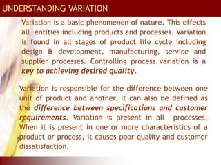
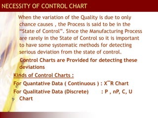
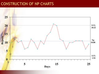
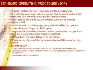
This document provides an overview of total quality management (TQM) concepts for manufacturing, including standard operating procedures (SOP), statistical process control (SPC), process capability indices, and control charts. It discusses how SOPs and quality control process charts are used to standardize operations and check quality. Statistical process control tools like control charts help monitor processes for variation. Process capability indices like Cp and Cpk indicate if a process is capable of meeting specifications. Together, these TQM elements aim to reduce variation and improve quality in manufacturing operations and supply chains.

1. TQM IN MANUFACTURING
Prof Yasutoshi Washio
(10th – 12th Sep 07

2. Agenda
• Understanding SOP / QCPC
• Understanding Statistical Process
Control : SPC, PMC, Cp, Cpk , Control
Charts
• Understanding Role of TQM in Supplier
Chain Management
• Understanding Role of TQM in Supply
Chain Management

3. What is SOP/QCPC

4. STANDARD OPERATING PROCEDURE (SOP)
• SOP is the contract between operator and the management.
• SOP must focus on how to do and not on what to do. It must contain
instruction 20 % on what to do and 80 % on how to do.
• Product quality should be built in through SOP and not through
operator’s skill.
• It should be written in language easily understood by the operator.
• It covers Plan and Do part of PDCA cycle.
• Changes in SOP should be done with active participation of operators
before perfection only comes through practicing.
• SOP should be religiously followed by operators.
• SOP is necessary to avoid the variation between shift, operator, day,
machine.
• Contents of SOP :
– Checking of equipment/ machine, material, etc. before starting of operations.
– It may cover some control points of control plan related to process and to be controlled
by operator.
– It may cover safety instructions.

5. QUALITY CONTROL PROCESS CHART (QCPC)
• QCPC specifies how to check and how to control.
• It covers check and act part of PDCA cycle to be followed by
supervisors and executives.
• SOP and PCPC are used for improvement in product quality.
• SOP and QCPC should be revised continuously through practicing
quality improvement tools.
• Limitations of SOP / QCPC : if the desirable results are not
achieved thru SOP /QCPC ,we have to consider
1. Design Change
2. Technology Change
3. POKA YOKE Introduction

6. STATISTICAL PROCESS CONTROL (SPC)

7. SPC , PROCESS CAPABILITY
The main objectives of SPC :
• To assess the stability of Process
• Removal of assignable causes
• Assess the capability of the process thru the use of Capability
Index Cp & Cpk
Necessity of Process Capability :
• Fraction of Quantitative Characteristics is no longer effective as an
index of Quality . There are two reasons for the same
1. High Quality of Products
2. Quality should be measured by distribution rather than
fraction defectives

8. 99.73% population between process mean +/- 3 SD
LSL USL
- 3 SD + 3 SD
2 3 4 5 6 7 8 9 12
10 16
15
14
13
11
1
PROCESS CAPABILITY
Cp = Tolerance
6 SD

9. PROCESS CAPABILITY INDEX
Interpretations of Cp
Cp > 1 : The process is quite capable
Cp = 1 : The process is just capable
Cp < 1 : The process is incapable
The recommended value of Cp is 1.33 ( minimum)
In order to achieve Six Sigma quality in the organization, we
must reduce the variation in the process so as to achieve the value of
Cp=2.

10. IMPACT & DRAW BACK OF PROCESS CAPABILITY
For individual parts, the ideal design is Cp = 2; in other words, the
design specification is twice as “wide” as the true capability of the
process. This is where the phrase “Six Sigma Quality” originated.
Since the process capability is +/- 3SD, a design specification twice
as wide would be +/- 6 SD.
Cp however is not a very reliable measure as it does not tell us all.
Consider the following four processes producing the same output X
with specification 20+/- 4. Each of these processes have the
Standard deviation of 1.
Impact of process capability :
Drawbacks of Cp :

11. LSL USL
X=20
SD=1
Cp=1.33
PROCESS 1 :

12. LSL USL
X=22
SD=1
Cp=1.33
PROCESS 2 ;

13. LSL USL
X=15
SD=1
Cp=1.33
PROCESS 3 :

14. LSL USL
X=25
SD=1
Cp=1.33
PROCESS 4 :

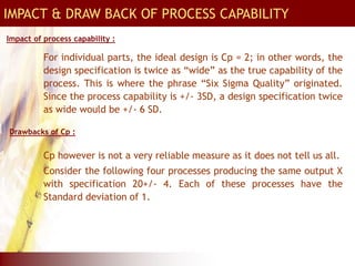
15. CALCULATION OF Cpk INDEX
Cpk is a measure of process performance capability
The process performance index Cpk is given by:-
Cpk = Min [ USL - x , x - LSL ]
3SD 3SD
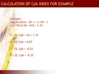
Example :
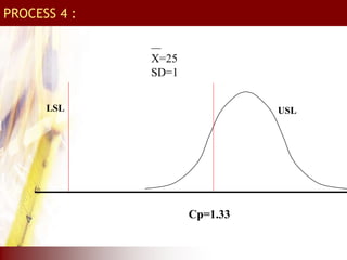
Specification : 20 +/- 4, SD = 1
Cp = Tolerance/6SD = 8/6 = 1.33

16. x = 20, Cpk = Cp = 1.33
x = 22, Cpk = 0.67
x = 15, Cpk = -0.33
x = 25, Cpk = -0.33
Example :
Specification : 20 +/- 4, SD = 1
Cp = Tol/6 SD = 8/6 = 1.33
CALCULATION OF Cpk INDEX FOR EXAMPLE

17. In the previous slide we observe that, although the Cp value =
1.33 in all the four cases, but because of the shift in the
process setting level we are getting Cpk values as 0.67 in 2nd
case and hence the non conformities. Similar observations are
noticed in 3rd and 4th case where we get the Cpk as -0.33.
Calculation of Cpk index
Thus Cpk = Cp means the process is centered.
Cpk < 1 means non- conformances are being produced.
Cpk < 0 indicates that the process has been set beyond
either of the two specification limits.
Note : Cpk is always less than or equal to Cp.
INTERPERATION OF THE EXAMPLE
INTERPERATION OF THE EXAMPLE

18. Therefore, the first step is to bring Cpk=Cp by proper
centering of the process. The second step should be to improve
the Cp value by decreasing the variation.
VARIOUS SIGMA LEVELS :
• In the chart below, 64.6% of the measures are between the
upper and lower limits
• This is a 1 sigma process
• Reducing the variations in the process will bring a higher
percentage within the acceptable limits
Mean (μ)
+1σ
-1σ
-2σ +2σ
-3σ +3σ
34.13 %
34.13 %
13.06 %
2.14 %
13.06 %
2.14 %
0.13 % 0.13 %
Lower
Limit
Upper
Limit
Cp & Cpk INDICES

19. CONTOL CHARTS

20. Suppliers Inputs
Process
Outputs
Business
Process
Critical
Customer
Requirements
Defects
Variation in output of processes
causes defects
UNDERSTANDING VARIATION

21. Variation is a basic phenomenon of nature. This effects
all entities including products and processes. Variation
is found in all stages of product life cycle including
design & development, manufacturing, service and
supplier processes. Controlling process variation is a
key to achieving desired quality.
UNDERSTANDING VARIATION
Variation is responsible for the difference between one
unit of product and another. It can also be defined as
the difference between specifications and customer
requirements. Variation is present in all processes.
When it is present in one or more characteristics of a
product or process, it causes poor quality and customer
dissatisfaction.

22. UNDERSTANDING & CONTROLING VARIATION
Products and processes are expected to vary because
no two things are exactly alike. Differences result
from material characteristics, methods, people,
machine and environmental factors as described on
the next slide.

23. Variation
Methods
•Procedures
•Policies
•Accounting
Material
•Assemblies
•Components
•Suppliers
•Consumables
Environment
•Noise level
•Humidity
•Temperature
•Lighting
People
•Training
•Experience
•Skill
•Attitude
Machine
•Technology
•Variability
•Tooling
•Fixtures
Measurement
•Counting
•Instruments
•Gauging
•Tests
SOURCES OF VARIATIONS

24. The Quality of manufactured products always subject to
certain amount of Variation. These Variation are mainly
due to two types of Causes.
Causes
Chance / Inherent Causes
They have the influence on
the output all the time.
Assignable Causes
They influence the output
only once in a while.
CAUSES OF VARIATION

25. When the variation of the Quality is due to only
chance causes , the Process is said to be in the
“State of Control”. Since the Manufacturing Process
are rarely in the State of Control so it is important
to have some systematic methods for detecting
serious deviation from the state of control.
Control Charts are Provided for detecting these
deviations
Kinds of Control Charts :
For Quantative Data ( Continuous ) : X¯R Chart
For Qualitative Data (Discrete) : P , nP, C, U
Chart
NECESSITY OF CONTROL CHART

26. Shift
Time
Date 1/1 1/2 1/3 1/4 1/5 1/6 1/7 1/8 1/9 1/10 1/11 1/12 1/13 1/14 1/15 1/16 1/17 1/18 1/19 1/20 1/21 1/22 1/23 1/24
X 1 54.00 52.00 51.00 55.00 56.00 56.00 54.00 54.00 56.00 48.00 54.00 52.00 51.00 55.00 56.00 56.00 54.00 54.00 56.00 48.00
X 2 55.00 51.00 52.00 53.00 55.00 52.00 52.00 53.00 51.00 53.00 55.00 51.00 52.00 53.00 55.00 52.00 52.00 53.00 51.00 53.00
X 3 51.00 46.00 49.00 50.00 48.00 52.00 49.00 49.00 46.00 48.00
X 4 50.00 47.00 52.00 48.00 49.00 51.00 49.00 52.00 45.00 50.00
X 5 II nd Ist
X 52.5 49 51 51.5 52 52.75 51 52 49.5 49.75 54.5 51.5 51.5 54 55.5 54 53 53.5 53.5 50.5 53.15 51.1
R 5 6 3 7 8 5 5 5 11 5 1 1 1 2 1 4 2 1 5 5 2.3 6
LSL- 46.73 (For X Chart) LSL- 48.9 (For X Chart)
Chart No. 01
Part No. MIQ 001 USL - 55.47 ( For X Chart) USL - 57.52 ( For X Chart)
Part Name. Round Bar
CONTROL LIMIT -1 CONTROL LIMIT -2
X CHART
LSL - 0.00 (For R Chart) LSL - 0.00 (For R Chart)
R = Average R = U.C.L = D4 R= L.C.L = ZERO R CHART
X = Average X = U.C.L = X + A 2 R L.C.L = X - A2 R
USL - 13.69 (For R Chart) USL - 7.51 (For R Chart)
42
43
44
45
46
47
48
49
50
51
52
53
54
55
56
57
58
59
0
1
2
3
4
5
6
7
8
9
10
11
12
13
14
15
EXAMPLE OF X¯R CHART

27. The p charts are used to control the overall number of
defective units in a process. The proportion of non
conforming items are plotted on this chart which gives
us the graphical display of variability of the data.
P CHARTS
CONSTRUCTION OF P CHART
The construction of control charts is very simple.
Simply select the range of data points ( “proportion”
column in the excel sheet ) and click the graph button.
Select “Line graph” and the p chart is automatically
calculated. The average, UCL and LCL can be manually
displayed by drawing three additional lines on the
graph. Please refer the next slide for the graph.

28. Day Rejects Tested Proportion
1 14 286 0.049
2 22 281 0.078
3 9 310 0.029
4 19 313 0.061
5 21 293 0.072
6 18 305 0.059
7 16 322 0.050
8 16 316 0.051
9 21 293 0.072
10 14 287 0.049
11 15 307 0.049
12 16 328 0.049
13 21 296 0.071
14 9 296 0.030
15 25 317 0.079
16 15 297 0.051
17 14 283 0.049
18 13 321 0.040
19 10 317 0.032
20 21 307 0.068
21 19 317 0.060
22 23 323 0.071
23 15 304 0.049
24 12 304 0.039
25 19 324 0.059
26 17 289 0.059
27 15 299 0.050
28 13 318 0.041
29 19 313 0.061
30 12 289 0.042
Total 493 9155
EX : CONSTRUCTION OF P CHART

29. Data points
Number of defective units
Number of units in the sample
P =
Process Average P =
Total defective units
Total units observed
Upper control Limit ( UCL ) = P+3 P ( 1-P )
n
Lower control Limit = P-3 P ( 1-P )
n
=
= 0.0926
=0.1508
0.053
FORMULES FOR P CHARTS

30. 0
0.01
0.02
0.03
0.04
0.05
0.06
0.07
0.08
0.09
0.1
5 15 25
LCL
0.015
UCL
0.0926
CL
0.053
Days
P CHART

31. NP CHART
The NP chart is used for
plotting number of defectives
instead of proportion
defectives. This is another
version of P chart and its
applicability depends upon the
interest of the end user.
Day Rejects Sample size
1 10 100
2 12 100
3 10 100
4 11 100
5 6 100
6 7 100
7 12 100
8 10 100
9 6 100
10 11 100
11 9 100
12 14 100
13 16 100
14 21 100
15 20 100
16 12 100
17 11 100
18 6 100
19 10 100
20 10 100
21 11 100
22 11 100
23 11 100
24 6 100
25 9 100
Total 272 2500
Example -construction of np charts

32. p = X1 + X2 + X3 +…..Xk
kn
n = subgroup sample size = 100
UCL = np + 3 np ( 1-p )
LCL = np - 3 np ( 1-p )
275
25*100
= = 0.1088
np = 0.1088*100 =10.88
=20.22
=1.54
FORMULES FOR NP CHART

33. 0
5
10
15
20
25
5 15 25
LCL
1.54
UCL
20.22
Np
10.88
Rejects
Days
CONSTRUCTION OF NP CHARTS

34. Thank you