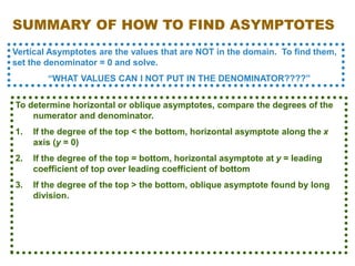
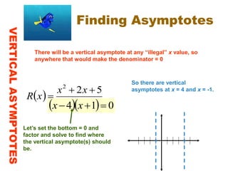
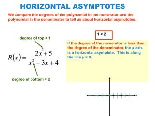
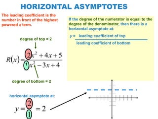
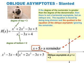
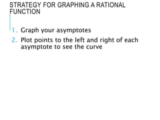
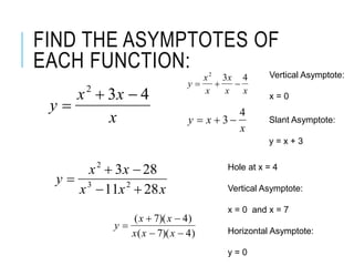
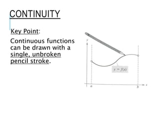
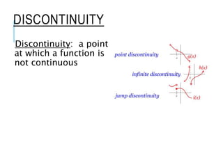
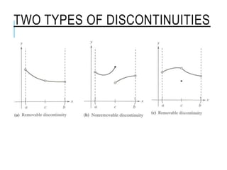
The document explains how to find vertical and horizontal or oblique asymptotes for rational functions, detailing the process of determining these using the degrees of the numerator and denominator. It also covers graphing strategies for rational functions, emphasizing the importance of asymptotes and points to consider when sketching the graph. Additionally, it discusses continuity and discontinuities in functions, addressing removable and non-removable discontinuities.

1. 8.3 RATIONAL FUNCTIONS
AND THEIR GRAPHS

2. SUMMARY OF HOW TO FIND ASYMPTOTES
Vertical Asymptotes are the values that are NOT in the domain. To find them,
set the denominator = 0 and solve.
“WHAT VALUES CAN I NOT PUT IN THE DENOMINATOR????”
To determine horizontal or oblique asymptotes, compare the degrees of the
numerator and denominator.
1. If the degree of the top < the bottom, horizontal asymptote along the x
axis (y = 0)
2. If the degree of the top = bottom, horizontal asymptote at y = leading
coefficient of top over leading coefficient of bottom
3. If the degree of the top > the bottom, oblique asymptote found by long
division.

3. Finding Asymptotes
VERTICAL
ASYMPTOTES
There will be a vertical asymptote at any “illegal” x value, so
anywhere that would make the denominator = 0
 
4
3
5
2
2
2





x
x
x
x
x
R
Let’s set the bottom = 0 and
factor and solve to find where
the vertical asymptote(s) should
be.
   0
1
4 

 x
x
So there are vertical
asymptotes at x = 4 and x = -1.

4. If the degree of the numerator is less than
the degree of the denominator, (remember
degree is the highest power on any x term)
the x axis is a horizontal asymptote.
If the degree of the numerator is less than
the degree of the denominator, the x axis
is a horizontal asymptote. This is along
the line y = 0.
We compare the degrees of the polynomial in the numerator and the
polynomial in the denominator to tell us about horizontal asymptotes.
 
4
3
5
2
2




x
x
x
x
R
degree of bottom = 2
HORIZONTAL ASYMPTOTES
degree of top = 1
1
1 < 2

5. If the degree of the numerator is equal to the
degree of the denominator, then there is a
horizontal asymptote at:
y = leading coefficient of top
leading coefficient of bottom
degree of bottom = 2
HORIZONTAL ASYMPTOTES
degree of top = 2
The leading coefficient is the
number in front of the highest
powered x term.
horizontal asymptote at:
1
2

 
4
3
5
4
2
2
2





x
x
x
x
x
R
1
2

y

6.  
4
3
5
3
2
2
2
3






x
x
x
x
x
x
R
If the degree of the numerator is greater
than the degree of the denominator, then
there is not a horizontal asymptote, but an
oblique one. The equation is found by
doing long division and the quotient is the
equation of the oblique asymptote ignoring
the remainder.
degree of bottom = 2
OBLIQUE ASYMPTOTES - Slanted
degree of top = 3
5
3
2 2
3


 x
x
x
4
3
2

 x
x
remainder
a
5

x
Oblique asymptote at y = x
+ 5

7. STRATEGY FOR GRAPHING A RATIONAL
FUNCTION
1. Graph your asymptotes
2. Plot points to the left and right of each
asymptote to see the curve

8. SKETCH THE GRAPH OF
10
5
3
2
)
(



x
x
x
f

9. 10
5
3
2
)
(



x
x
x
f
The vertical asymptote is x = -2
The horizontal asymptote is y = 2/5

10. 10
5
3
2
)
(



x
x
x
f
-10 -8 -6 -4 -2 2 4 6 8 10
-10
-8
-6
-4
-2
2
4
6
8
10

11. SKETCH
THE GRAPH
OF:
g(x) 
1
x 1
Vertical asymptotes at??
x = 1
Horizontal asymptote at??
y = 0

12. SKETCH
THE GRAPH
OF:
f (x) 
2
x
Vertical asymptotes at??
x = 0
Horizontal asymptote at??
y = 0

13. SKETCH
THE GRAPH
OF:
h(x) 
4
x
Vertical asymptotes at??
x = 0
Horizontal asymptote at??
y = 0

14. SKETCH
THE GRAPH
OF:
y 
1
x  3
 2
Vertical asymptotes at?? x = 1
Horizontal asymptote at?? y = 0
Hopefully you remember,
y = 1/x graph and it’s asymptotes:
Vertical asymptote: x = 0
Horizontal asymptote: y = 0

15. OR…
We have the function:

y 
1
x  3
 2
But what if we simplified this and combined like terms:
y 
1
x  3

2(x  3)
x  3
y 
1 2x  6
x  3
y 
2x  5
x  3
Now looking at this:
Vertical Asymptotes??
x = -3
Horizontal asymptotes??
y = -2

16. SKETCH
THE GRAPH
OF:
h(x) 
x2
 3x
x
Hole at??
x = 0
h(x) 
x(x  3)
x

17. FIND THE ASYMPTOTES OF
EACH FUNCTION:
y 
x2
 3x  4
x

y 
x2
 3x  28
x3
11x2
 28x

y 
x2
x

3x
x

4
x

y  x  3 
4
x
Slant Asymptote:
y = x + 3
Vertical Asymptote:
x = 0
y 
(x  7)(x  4)
x(x  7)(x  4)
Hole at x = 4
Vertical Asymptote:
x = 0 and x = 7
Horizontal Asymptote:
y = 0

18. WHAT MAKES A FUNCTION
CONTINUOUS?
Continuous functions are predictable…
1) No breaks in the graph
A limit must exist at every x-value or
the graph will break.
2) No holes or jumps
The function cannot have undefined
points or vertical asymptotes.

19. CONTINUITY
Key Point:
Continuous functions
can be drawn with a
single, unbroken
pencil stroke.

20. CONTINUITY OF POLYNOMIAL
AND RATIONAL FUNCTIONS
A polynomial function is continuous at every real
number.
A rational function is continuous at every real
number in its domain.

21. DISCONTINUITY
Discontinuity: a point
at which a function is
not continuous

22. DISCONTINUITY
Two Types of Discontinuities
1) Removable (hole in the graph)
2) Non-removable (break or vertical asymptote)
A discontinuity is called removable if a function can
be made continuous by defining (or redefining) a
point.

23. TWO TYPES OF DISCONTINUITIES

24. DISCONTINUITY
2
2
( )
3 10
x
f x
x x


 
Find the intervals on which these function are
continuous.
2
( 2)( 5)
x
x x


 
1
( 5)
x


Point of discontinuity:
2 0
x  
2
x  
Vertical Asymptote:
5 0
x  
5
x 
Removable
discontinuity
Non-removable
discontinuity

25. DISCONTINUITY
2
2
( )
3 10
x
f x
x x


 
( , 2) ( 2, 5) (5, )
     
Continuous on:

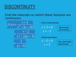
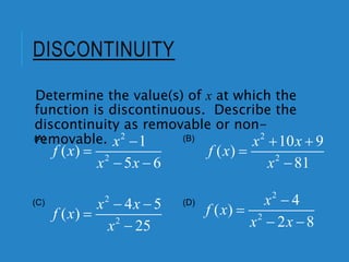
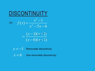
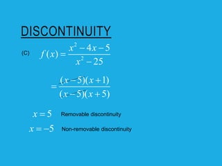
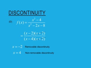
26. DISCONTINUITY
2
2 , 2
( )
4 1, 2
x x
f x
x x x
 

 
  

2
lim( 2 )
x
x



2
2
lim( 4 1)
x
x x


 
(2)
f
4
 
3
 
4
 
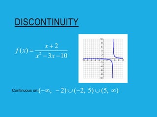
( , 2] (2, )
  
Continuous on:

27. DISCONTINUITY
Determine the value(s) of x at which the
function is discontinuous. Describe the
discontinuity as removable or non-
removable. 2
2
1
( )
5 6
x
f x
x x


 
2
2
4 5
( )
25
x x
f x
x
 


2
2
10 9
( )
81
x x
f x
x
 


2
2
4
( )
2 8
x
f x
x x


 
(A) (B)
(C) (D)

28. DISCONTINUITY
2
2
1
( )
5 6
x
f x
x x


 
(A)
( 1)( 1)
( 6)( 1)
x x
x x
 

 
1
x  
6
x 
Removable discontinuity
Non-removable discontinuity

29. DISCONTINUITY
(B)
9
x  
9
x 
Removable discontinuity
Non-removable discontinuity
( 9)( 1)
( 9)( 9)
x x
x x
 

 
2
2
10 9
( )
81
x x
f x
x
 



30. DISCONTINUITY
(C)
5
x 
5
x  
Removable discontinuity
Non-removable discontinuity
( 5)( 1)
( 5)( 5)
x x
x x
 

 
2
2
4 5
( )
25
x x
f x
x
 



31. DISCONTINUITY
(D)
2
x  
4
x 
Removable discontinuity
Non-removable discontinuity
( 2)( 2)
( 4)( 2)
x x
x x
 

 
2
2
4
( )
2 8
x
f x
x x


 

32. CONCLUSION
Continuous functions have no breaks, no holes, and no
jumps.
If you can evaluate any limit on the function using only
the substitution method, then the function is continuous.