1. MAS230 : Biostatistical Methods
Tutorial 4
SPSS Guidelines
• If you have not completed Tutorial 3, please do so before beginning Tutorial 4.
• Kappa Test and McNemar’s Test Revisited:
– Last week, we examined how to carry out a kappa test or McNemar’s test
if we have totals for a 2 × 2 table. This required that we use 0s and 1s to
represent rows and columns and then weight each unique combination of 0s
and 1s by the corresponding quantity in the table. In essence, these weights
created replicates for each of the unique 0-1 combinations.
∗ e.g. Consider the table we examined last week. The top left cell corre-
30 20
20 40
sponds to a row value of ‘0’ and a column value of ‘0’. When we weighted
by cases, this cell was given a weight of 30. In essence, SPSS created 30
separate entries with a row value of ‘0’ and a column value of ‘0’, even
though this does not appear anywhere.
– Suppose that, instead of a table like the one above, we are simply given 0-1
variables values for each person. These 0-1 variables correspond to a row and
column of a table of total counts. Instead of having the totals counts falling
in each cell, however, we have the individual data used to produce those total
counts. In this case, we can replicate the analysis we did last week, but we
no longer need to weight by cases since the data we have are essentially the
expanded version of the table.
– Select: Analyze −→ Descriptive Statistics −→ Crosstabs · · · and input
the variable corresponding to the rows and variable corresponding to columns
– Click the Statistics button and tick the boxes for Kappa or McNemar
– These instructions apply to other common analyses for tables, including chi-
square tests.
• You should be able to carry out all other analyses using the instructions provided
in the course reader and previous tutorials.
1

2. R Guidelines
• If you have not completed Tutorial 3, please do so before beginning Tutorial 4.
• Recall that you will need to determine the location of data files when you save
them to your computer (e.g., “C:Documents and Settings · · · dataset3.sav.” Re-
member that you will need to report this file location to R as “C:Documents and
Settings · · · dataset3.sav” for R to read the file). To determine this, you may
need to right-click on the file and select Properties. For Mac users, you will need
to command-click on the file and select Get Info.
• Remember that, to open SPSS data files, you will need to load the foreign package
by running the code:
> library(foreign)
The following code will read in the data to the variable “dataset3” after you replace
my file location with the correct file location on your computer:
> dataset3 <- read.spss(‘‘/Users/ryan/Documents/MAS230/dataset3.sav’’)
To access the variables, run the code:
> attach(dataset3)
• Recall from previous tutorials that Wilcoxon signed-rank tests and Mann-Whitney
U tests can be carried out using the function wilcox.test(), sign tests can be car-
ried out using the binom.test() function, and t-tests (one-sample, paired, and two-
sample) can be carried out using the function t.test(). Type in ?wilcox.test,
?binom.test(), or ?t.test() to see R’s help file on these particular functions.
• Instructions for Q-Q plots, bar charts, kappa tests, and McNemar’s test are provided
in the previous tutorial.
• Tests for Independent Proportions:
Tests for two independent proportions can be carried out using the prop.test()
function. This requires that you specify the number of successes for the two samples
as well as the sample sizes. Suppose we had two samples of size 25 and 30, and we
observed 10 successes in the first sample, and 18 successes in the second sample.
Further suppose that we wanted to test the hypotheses
H0 : π1 = π2
H1 : π1 < π2
We could carry out the test by running the following code:
2

3. > prop.test(x = c(10, 18), n = c(25, 30), alternative = "less", correct
= FALSE)
2-sample test for equality of proportions without continuity correction
data: c(10, 18) out of c(25, 30)
X-squared = 2.1825, df = 1, p-value = 0.06979
alternative hypothesis: less
95 percent confidence interval:
-1.00000000 0.01821449
sample estimates:
prop 1 prop 2
0.4 0.6
Thus, the p-value is 0.06979. Note that this uses a normal approximation, but it
reports a χ2 test statistic. To get the z-statistic, we can simply take the square root
√
of the χ2 test statistic, so the test statistic is given by z = 2.1825 = 1.477329.
• Chi-Square Tests:
To carry out a chi-square test, use the function chisq.test(). Suppose we have the
table of counts for assignment of males and females to treatment and control groups,
and we want to determine whether assignment to treatment or control is associated
with sex (i.e. probability of being assigned to treatment or control changes based on
your sex). To carry out a chi-square test of independence, we first must construct
Treatment Control
Male 30 20
Female 20 40
a matrix (think of this as being like a table) for the counts in the table. Running
the code
> x <- matrix(c(30, 20, 20, 40), nrow = 2, ncol = 2, byrow = TRUE)
creates a matrix with two rows and two columns, and it fills in this matrix with the
numbers 30, 20, 20, and 40 by going across the rows (instead of down the columns).
Running the code
> chisq.test(x, correct = FALSE)
Pearson’s Chi-squared test
data: x
X-squared = 7.8222, df = 1, p-value = 0.005161
3

4. carries out a chi-square test and reports a test statistic of χ2 = 7.8222 with a p-value
of 0.005161.
• Fisher’s Exact Test:
To perform Fisher’s exact test, use the function fisher.test(). This requires a
matrix specification in the same format as for the chi-square test. Running the code
> fisher.test(x)
Fisher’s Exact Test for Count Data
data: x
p-value = 0.007045
alternative hypothesis: true odds ratio is not equal to 1
95 percent confidence interval:
1.283785 7.051709
sample estimates:
odds ratio
2.968567
carries out Fisher’s exact test and produces a p-value of 0.007045.
• Levene’s Test:
To carry out Levene’s test, you will first need to install the car package if you are
working from your home computer. (If you do not recall how to do this, refer back
to Tutorial 1, where directions were given for installing the foreign package.) Once
you have installed the car package, you can load it by running
> library(car)
Levene’s test can then be carried out by using the leveneTest() function (specified
as levene.test() in older versions of R). Before using this function, however, you
need to first carry out a linear regression using the lm() function. You must take
all of your columns and save them to one variable (I’ll call this outcome), and then
you should create a second variable that records the group to which each outcome
corresponds (I’ll call this group). Then running the following code
> lm(outcome ∼ factor(group))
will carry out a linear regression of outcome on the different group categories. The
dependent variable is specified on the left of the ‘∼,’ and the independent variable
(or variables) is specified to the right of the ‘∼.’ We will need to save the regression
in a variable that is then passed as an argument to the leveneTest function,
> model <- lm(outcome ∼ factor(group))
> leveneTest(model)
4

5. – Note that the output from Levene’s test is slightly different for SPSS and R.
This is because SPSS uses absolute deviations from the mean, whereas R uses
absolute deviations from the median.
• After completing the tutorial, you will want to compare your R code to mine to
better understand any differences in output. You will also want to check your
solutions.
5

6. Questions
1. Consider Data Set 75. These data come from Judge, M.D. et al (1984). “Thermal
shrinkage temperature of intramuscular collagen of bulls and steers,” Journal of
Animal Science 59: 706–9, and are reproduced in Samuels and Witmer (1999),
Statistics for Life Sciences, 2nd Edition, Prentice Hall, p. 357. The study is designed
to assess the effect of electrical stimulation of a beef carcass in terms of improving
the tenderness of the meat. In this test, beef carcasses were split in half. One
side was subjected to a brief electrical current while the other was an untreated
control. From each side a specimen of connective tissue (collagen) was taken, and
the temperature at which shrinkage occurred was determined. Increased tenderness
is related to a low shrinkage temperature.
Carry out analyses to assess the impact of electrical stimulation on the meat tender-
ness. Use both parametric and non-parametric methods and compare the results.
Suppose acceptable tenderness corresponds to a shrinkage temperature less than
69 degrees. How would you test to see if the proportions of acceptable tenderness
values differed under the two treatments? Use SPSS to create appropriate variables
to enable this to be tested and carry out the analysis. Don’t forget that the sample
sizes are small here.
2. Refer to Data Set 76. These data come from Mochizuki, M. et al (1984). “Effects
of smoking on fetoplacentalmaternal system during pregnancy,” American J. Ob-
stet. Gyn. 149: 13–20. The study considered the effects of smoking during preg-
nancy by examining the placentas from 58 women after childbirth. Each mother was
classified as a non-, moderate or heavy smoker during pregnancy, and the outcome
measure was presence or absence of atrophied placental villi, finger-like structures
that protrude from the wall to increase absorption area.
Combine the two smoking classes to create a “smoker” class and carry out an
appropriate test for association of villi atrophy with smoking status. (Note to SPSS
users: This means that you will have to use Transform → Compute Variable. . .
to create a new variable. Since smoker status is denoted by characters [H, M, N],
you will need to use quotes around these in the “Numeric Expression:” box.)
Given there are three ordered classes of smoking (none < moderate < heavy) think
about how you might display such data.
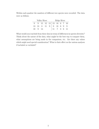
3. An environmental scientist studying the impact of pollution on species diversity
along two nearby rivers carried out a survey in which plots (quadrats) of size 30
metres by 20 metres were randomly chosen from along the banks of the rivers.
6

7. Within each quadrat the numbers of different tree species were recorded. The data
were as follows:
Valley River Ridge River
9 9 15 12 13 13 10 6 7 10
13 13 8 11 9 9 18 6 9 9
10 9 14 11 7 8 6 11
What would you conclude from these data in terms of differences in species diversity?
Think about the nature of the data, what might be the best way to compare them,
what assumptions are being made in the comparison, etc. Are there any values
which might need special consideration? What is their effect on the various analyses
if included or excluded?
7