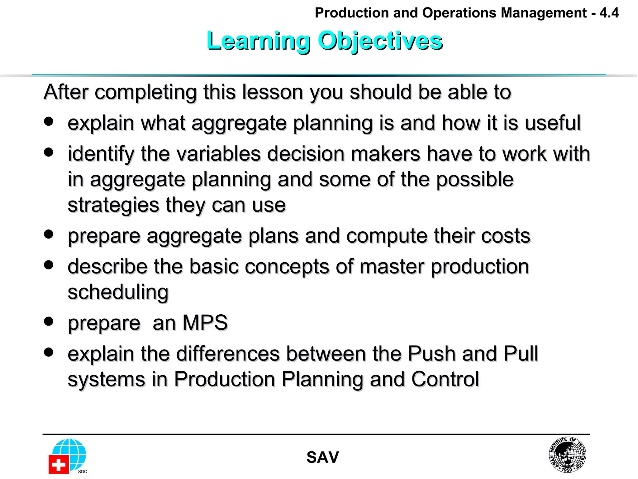
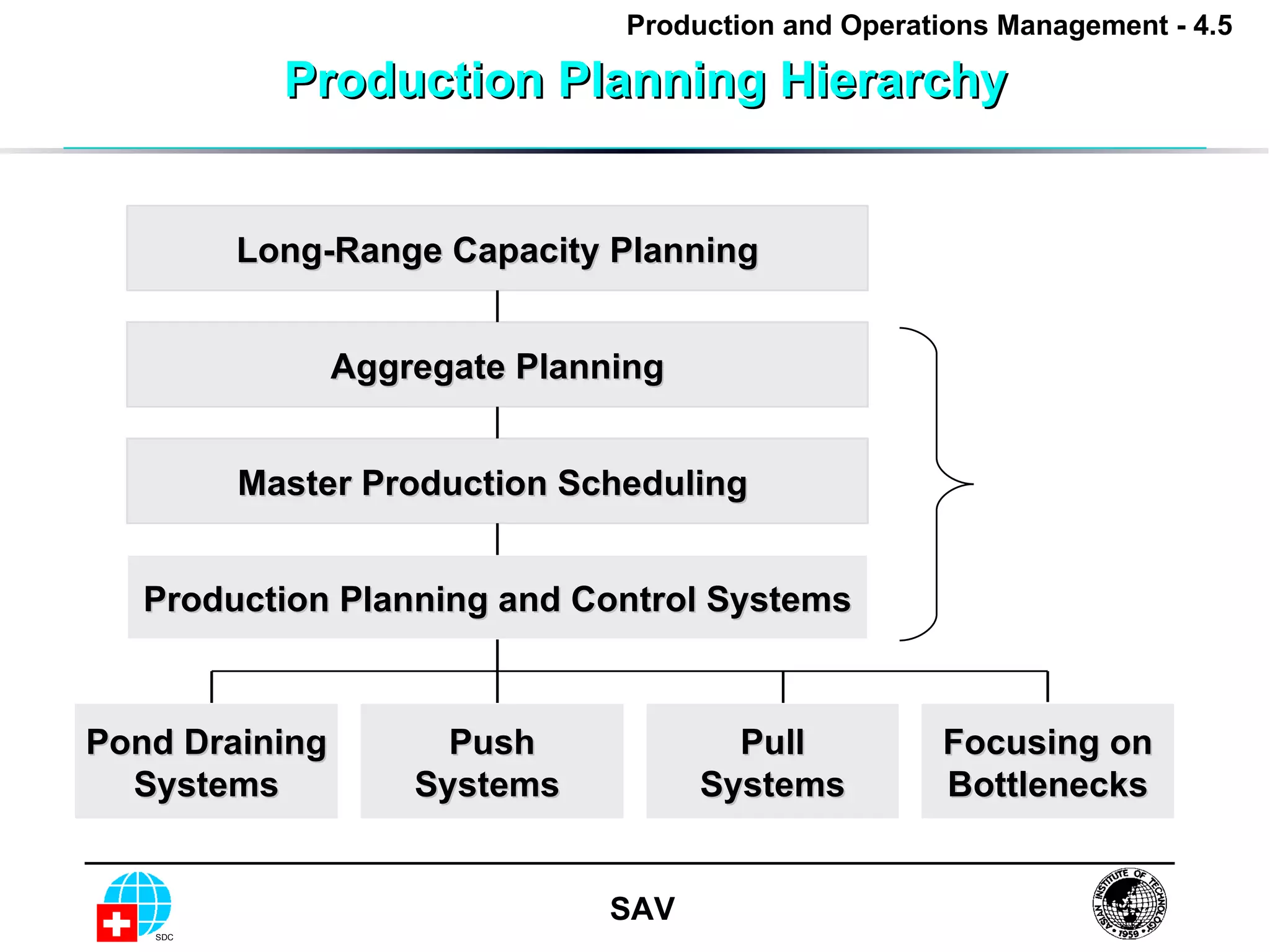
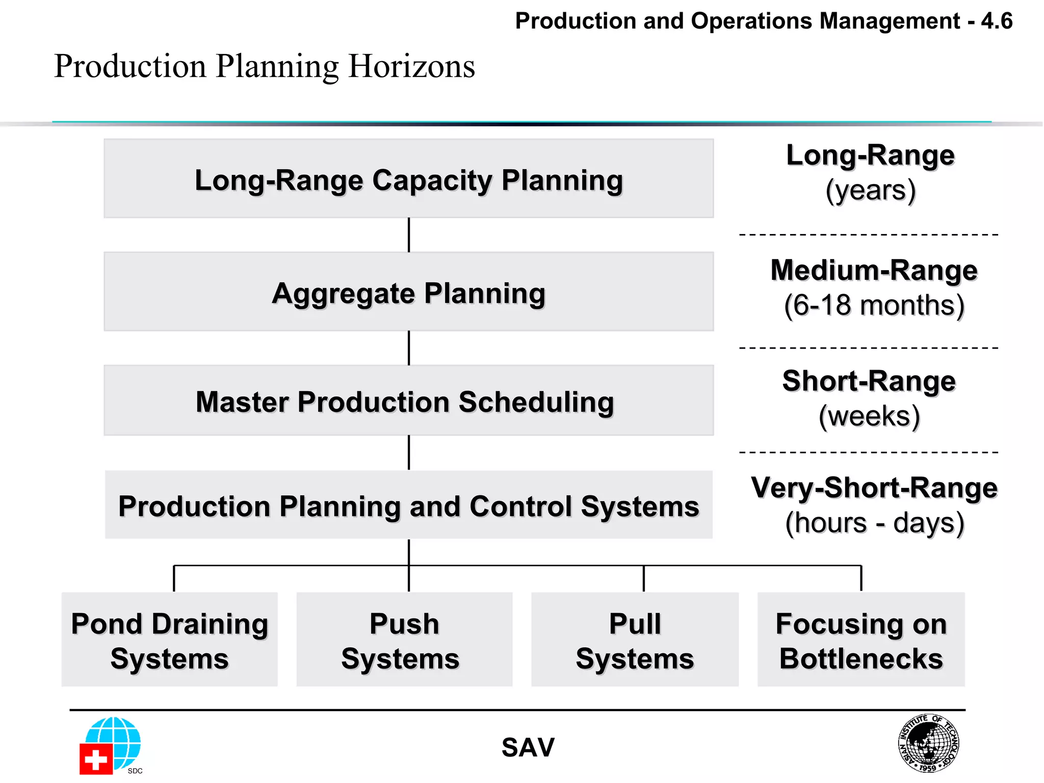
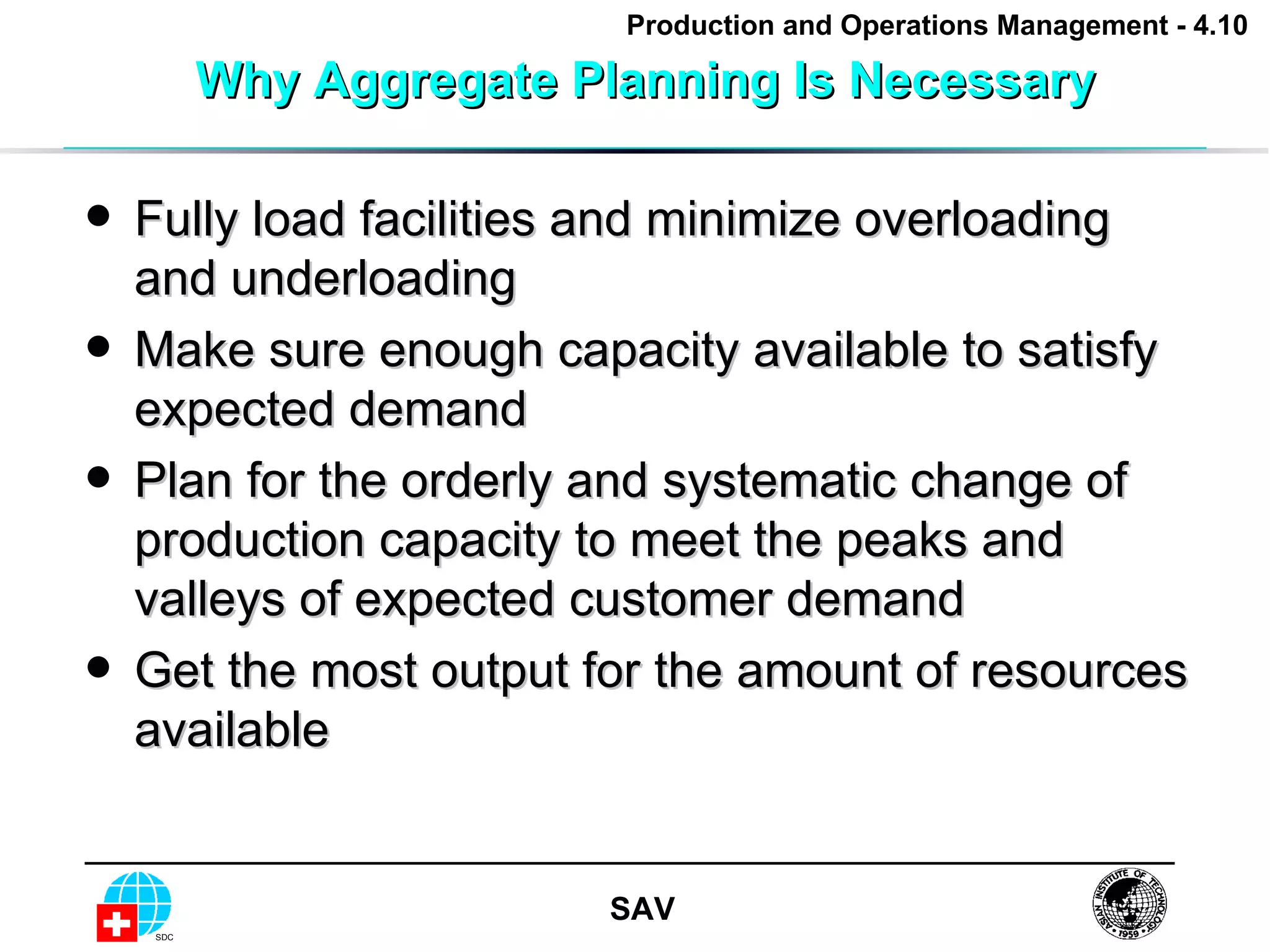
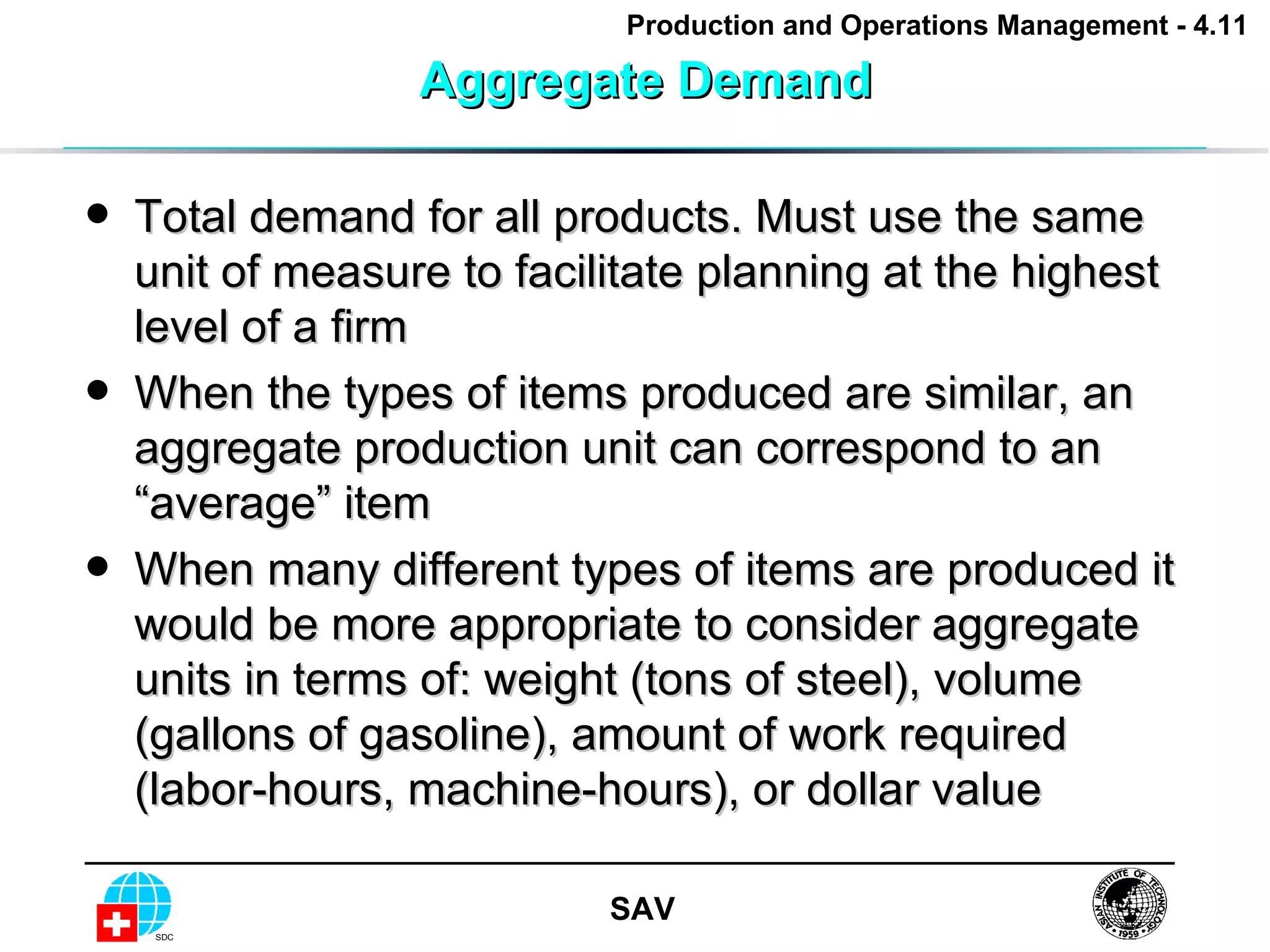
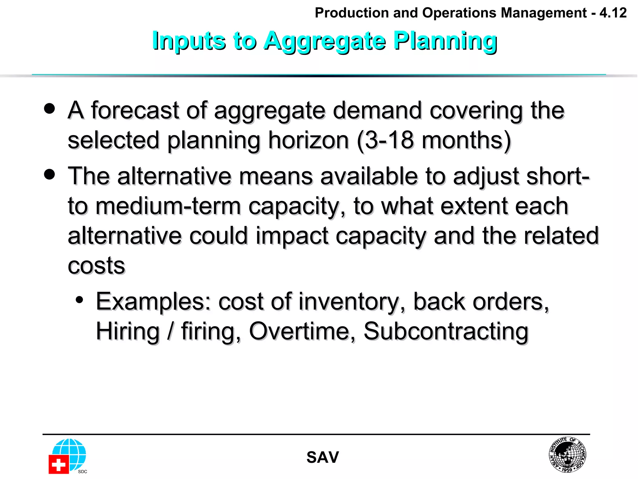
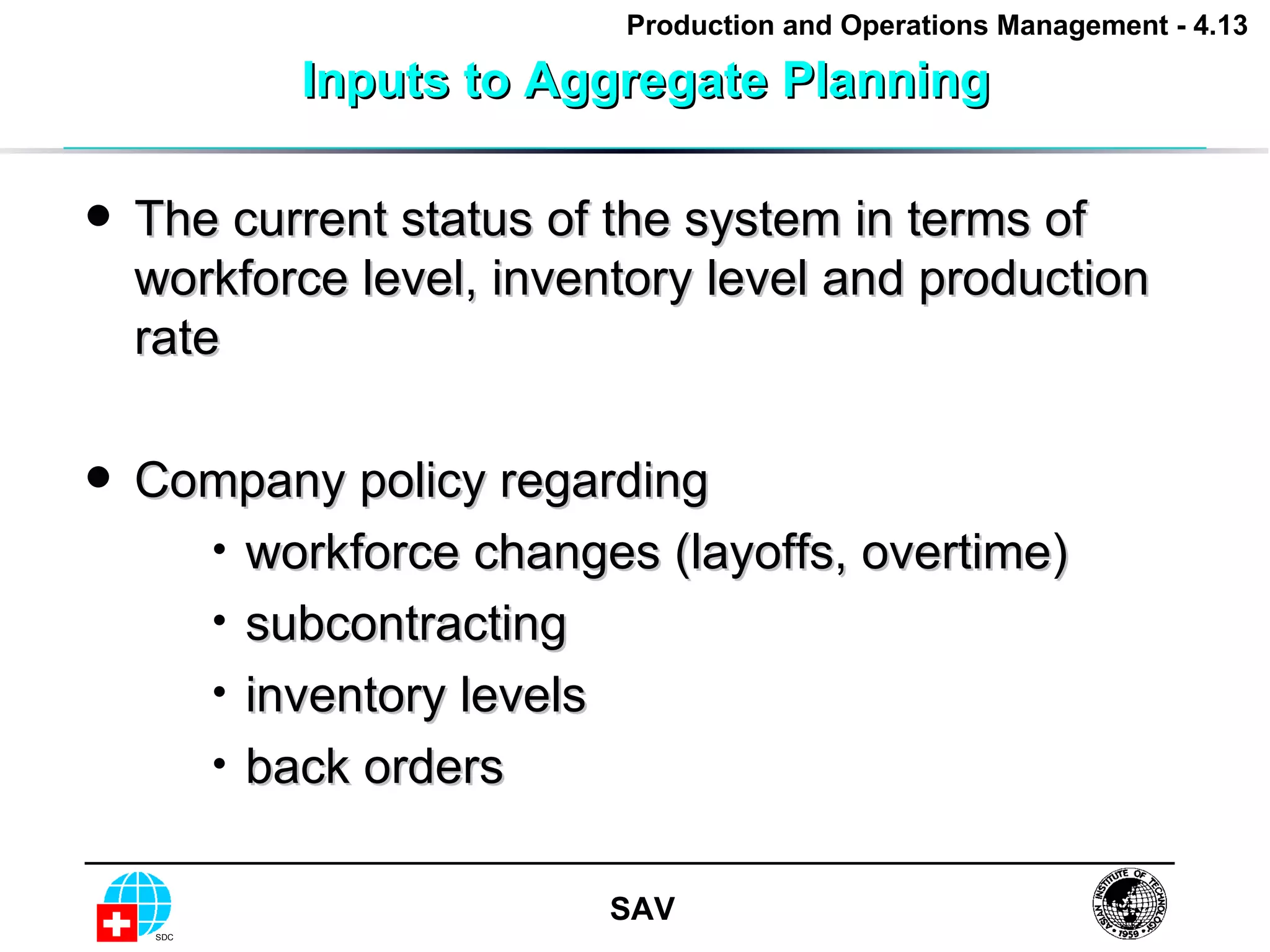
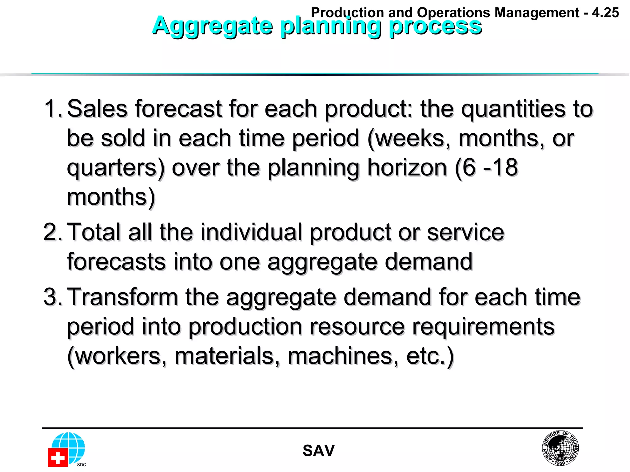
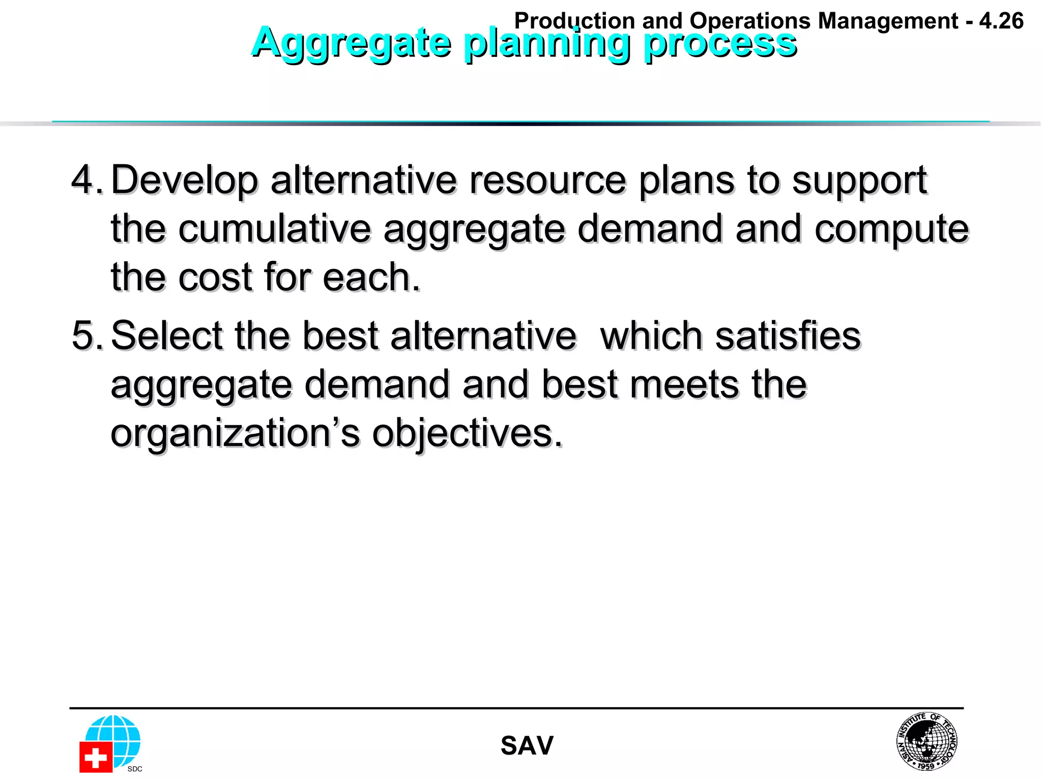
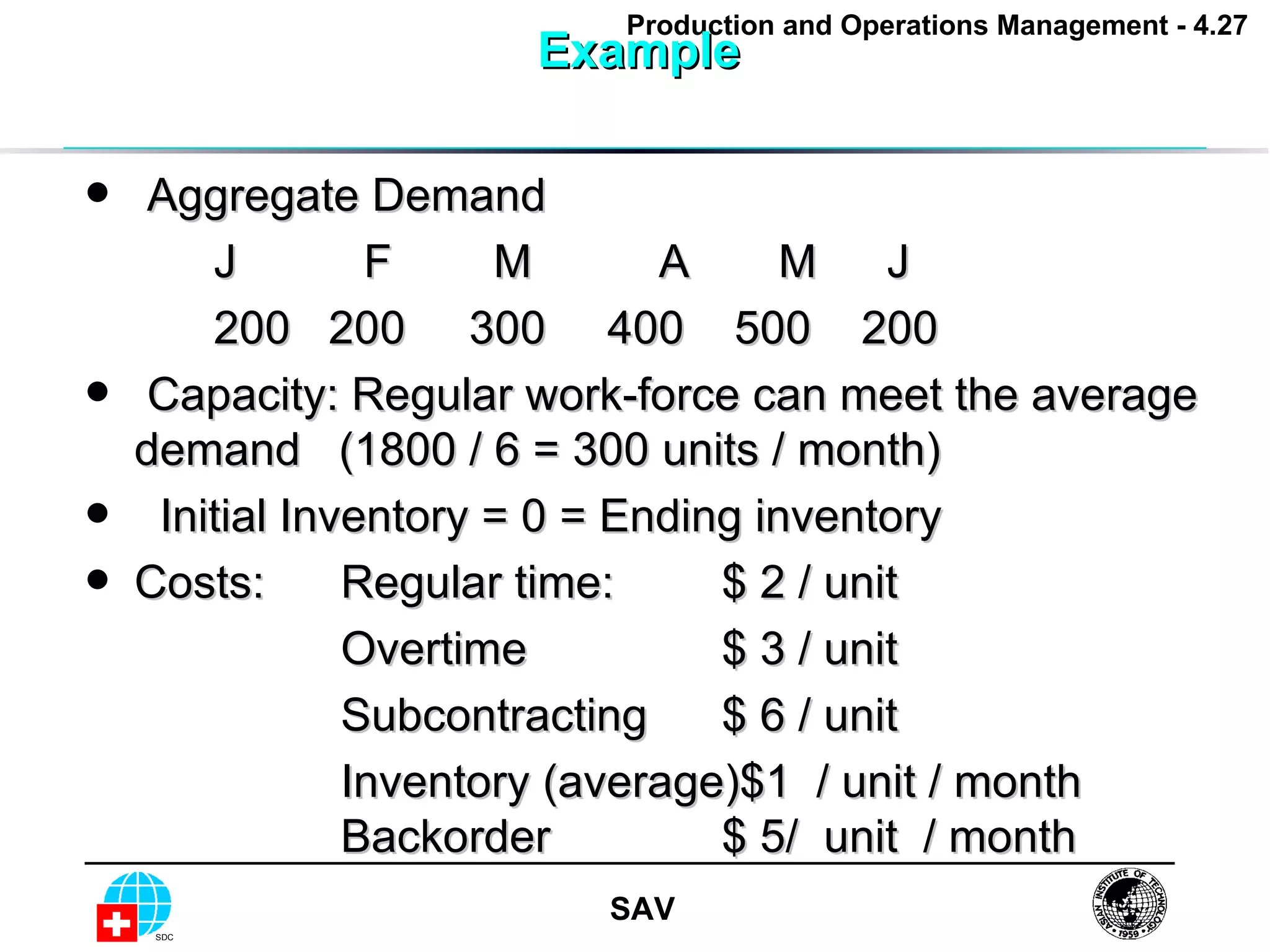
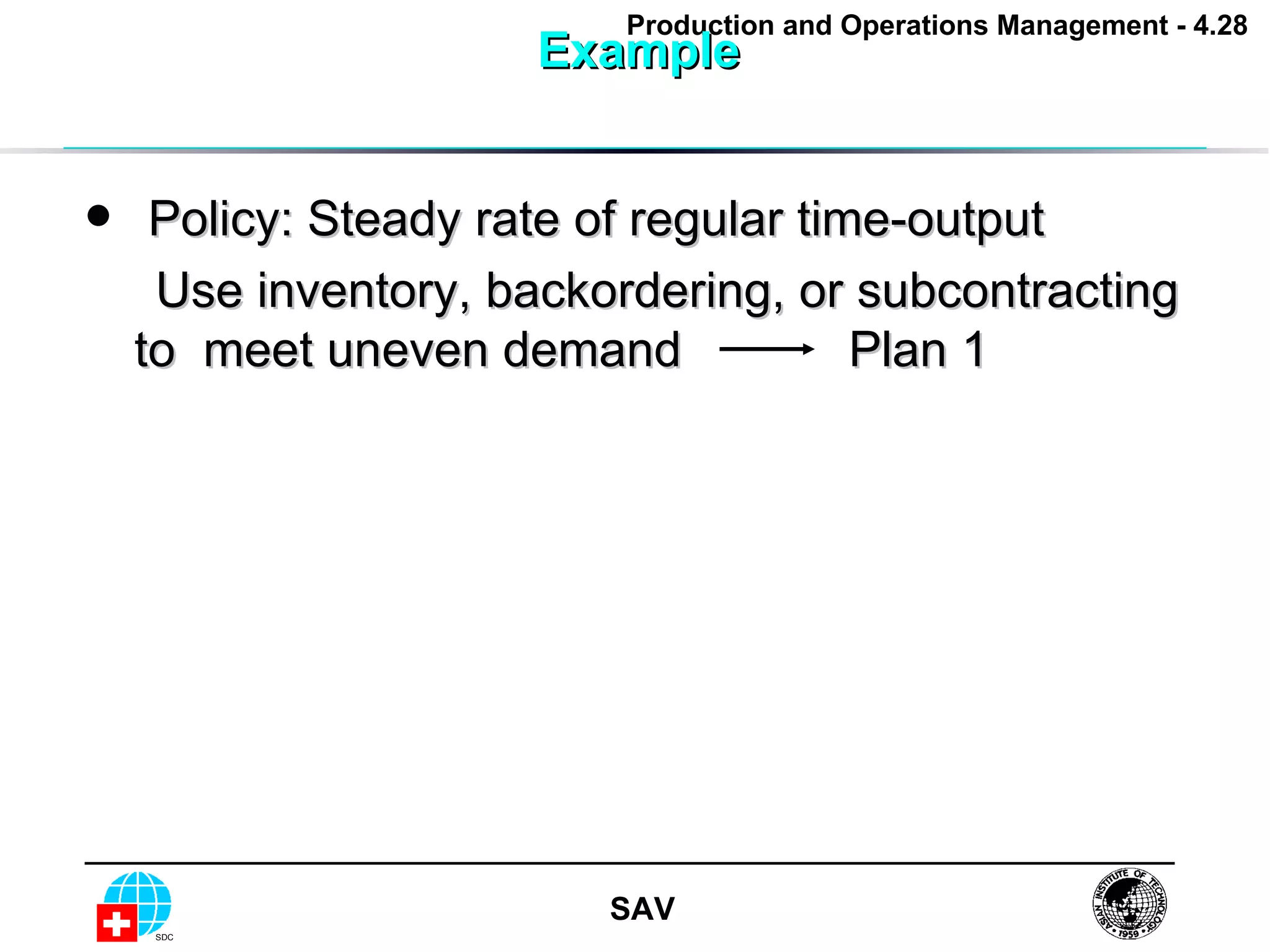
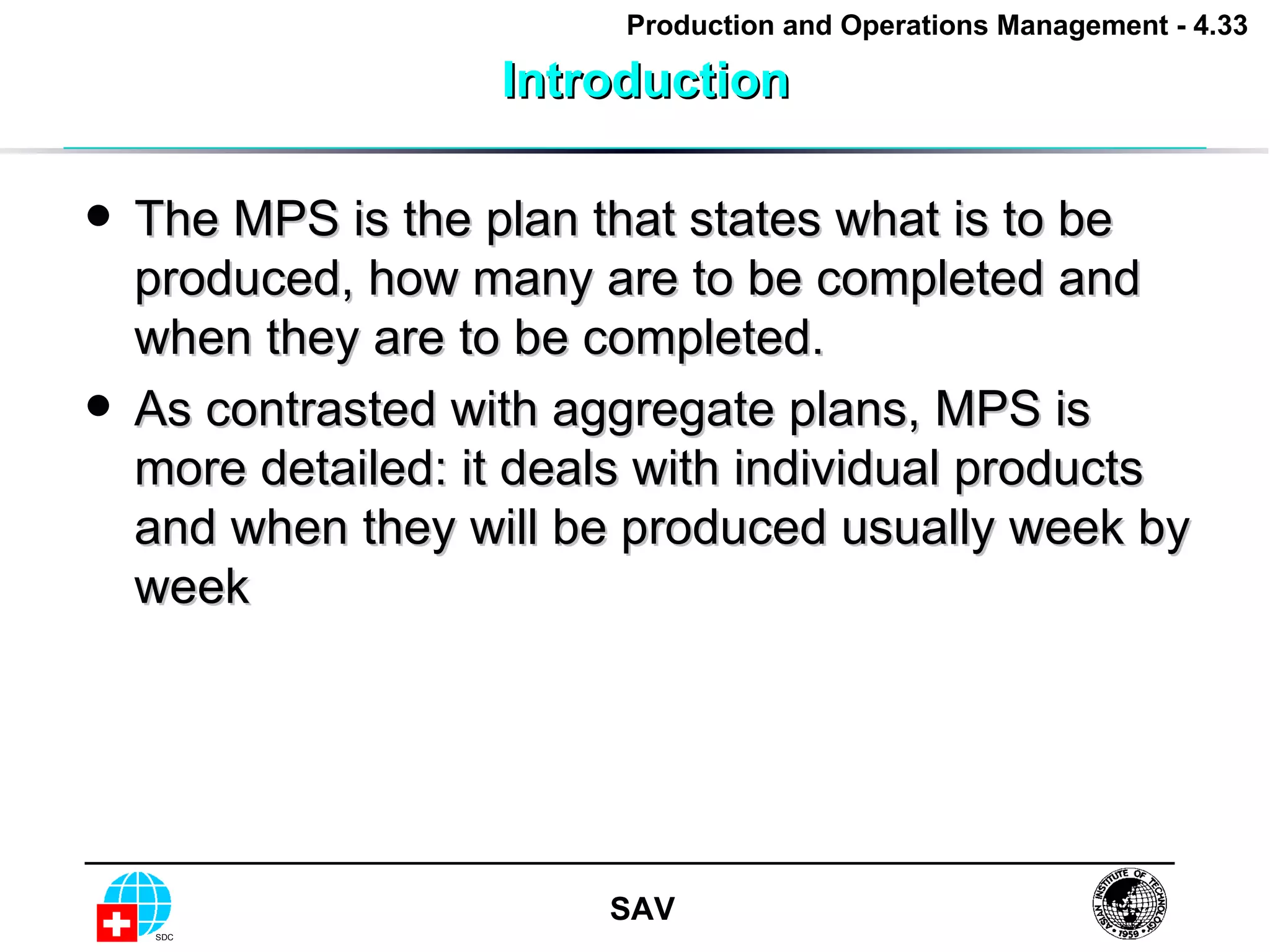
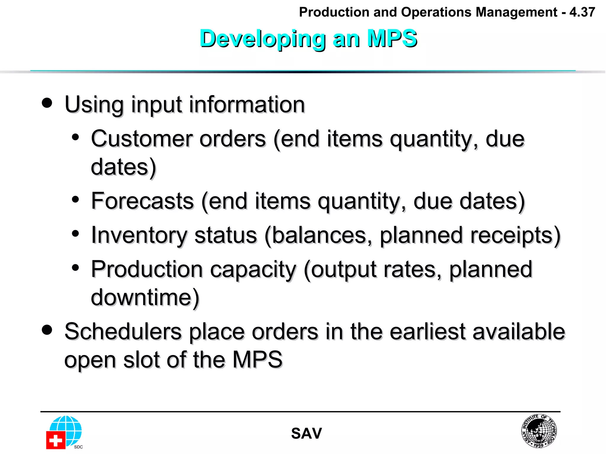
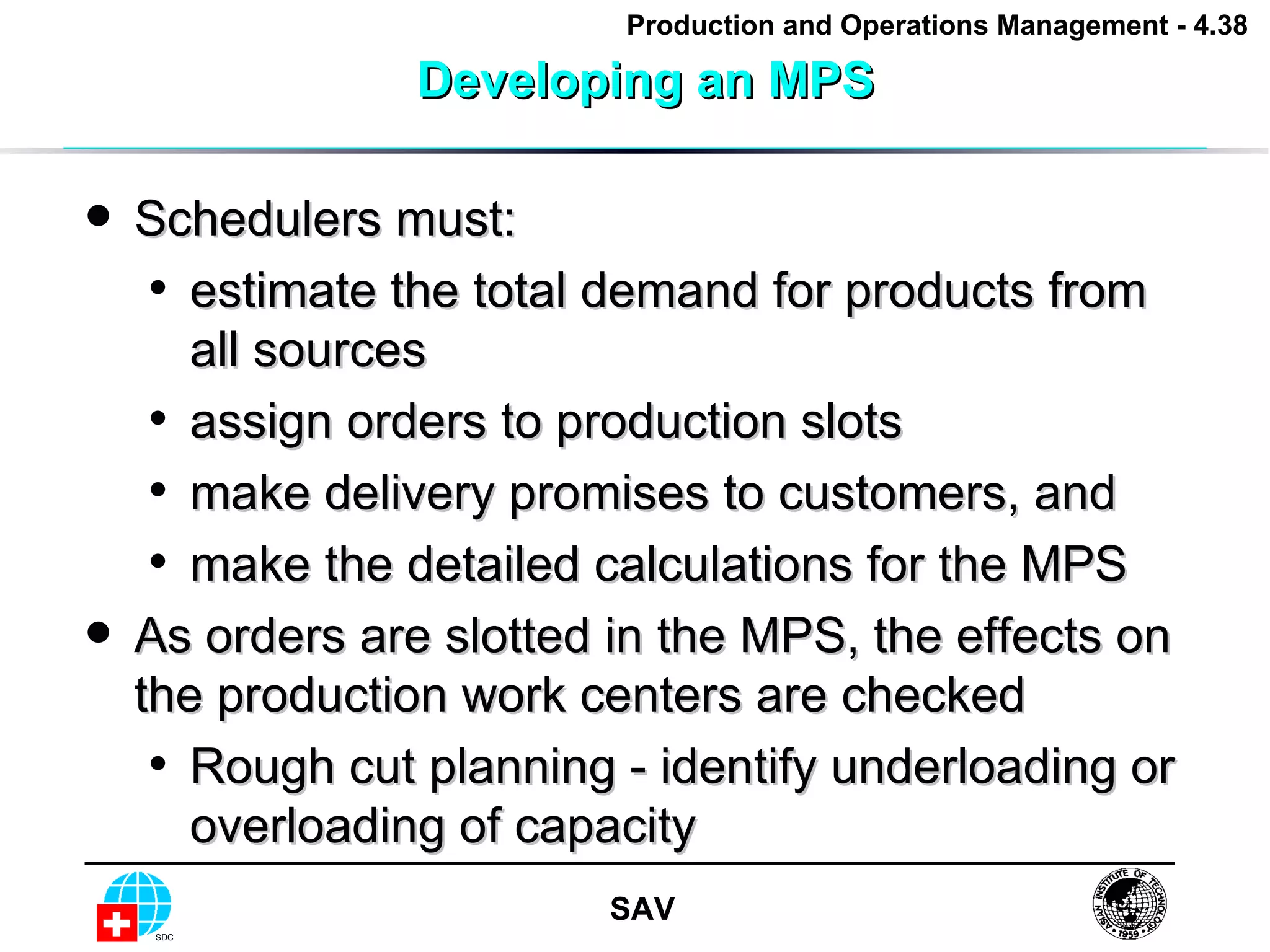
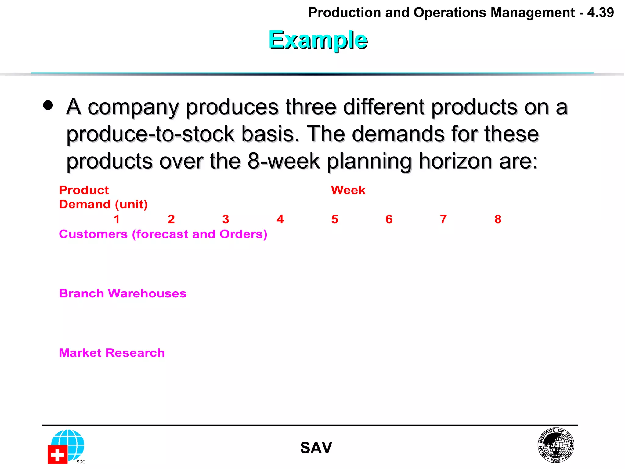
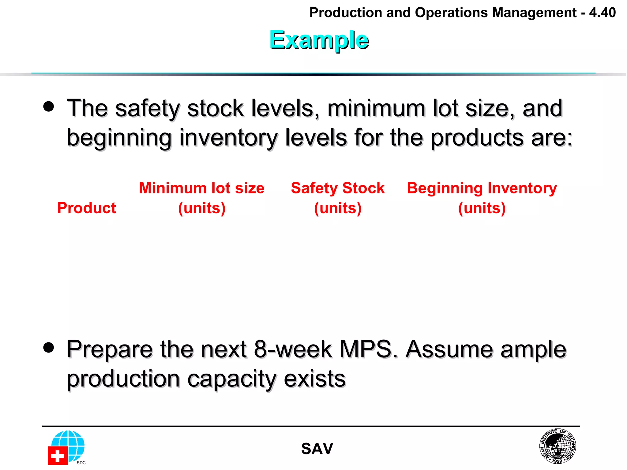
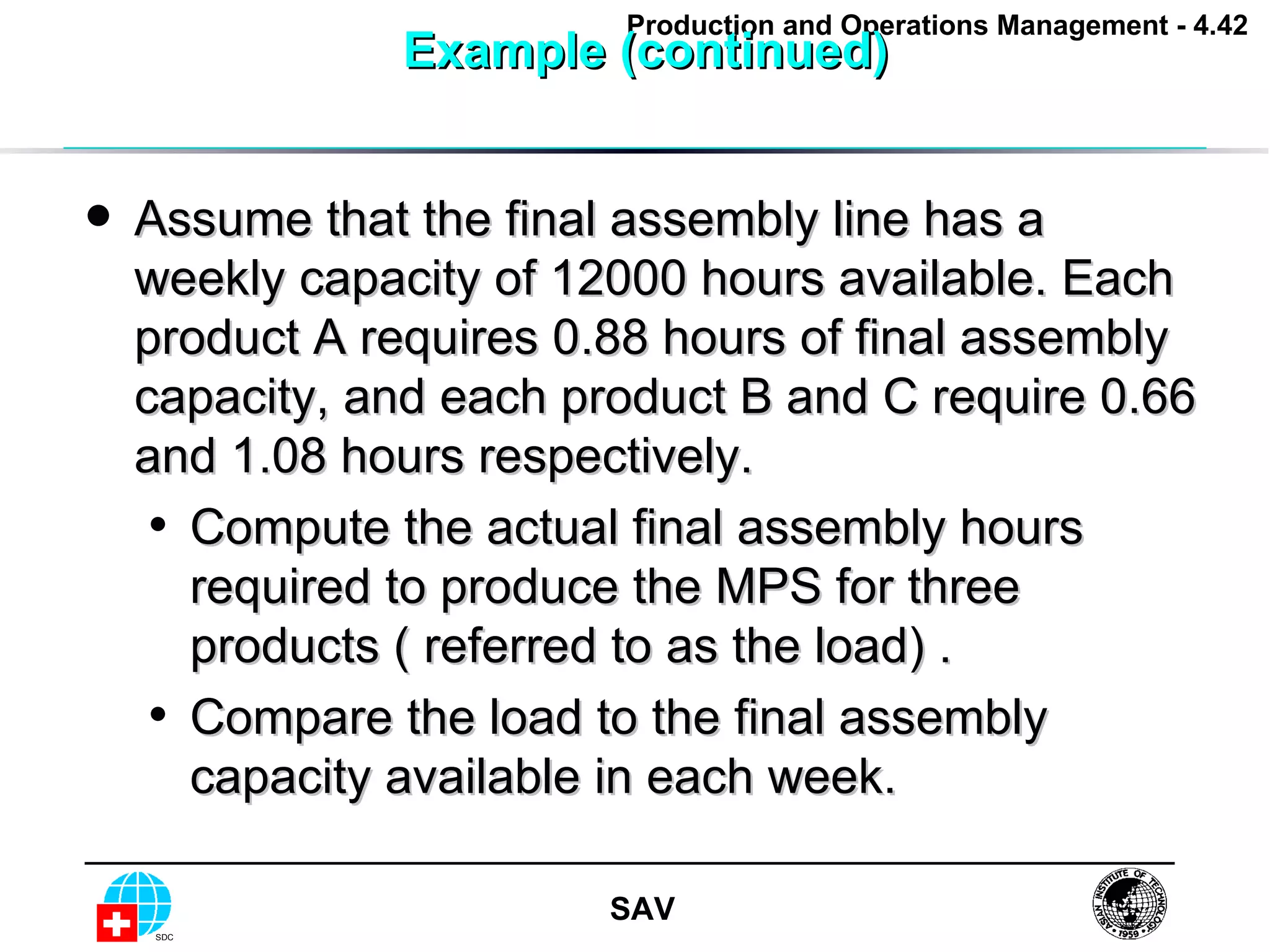
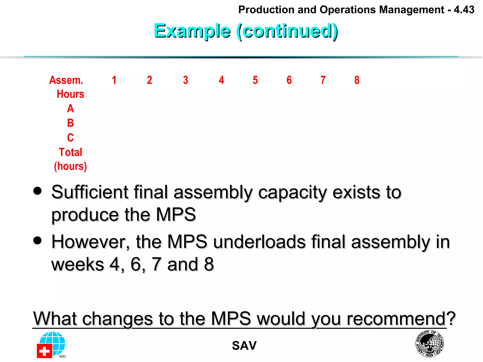
The document discusses production planning systems including aggregate planning and master production scheduling. It provides an overview of different planning horizons and techniques for aggregate and master production scheduling. An example is given demonstrating how to develop a master production schedule over an 8 week planning horizon for 3 products considering demand forecasts, safety stocks and production capacity.

1. Lesson 4 Production-Planning Systems: Aggregate Planning and Master Production Scheduling

2. Overview Production-Planning Hierarchy Aggregate Planning Master Production Scheduling Types of Production-Planning and Control Systems

3. Lesson 4 Readings: Textbook: chapter 9 Homework : Review and discussion questions: 4, 5, 7, 8, 9, 15, 18, 19 Problems: 1, 3, 4, 8, 9, 10, 14, 15

4. Learning Objectives After completing this lesson you should be able to explain what aggregate planning is and how it is useful identify the variables decision makers have to work with in aggregate planning and some of the possible strategies they can use prepare aggregate plans and compute their costs describe the basic concepts of master production scheduling prepare an MPS explain the differences between the Push and Pull systems in Production Planning and Control

5. Production Planning Hierarchy Master Production Scheduling Production Planning and Control Systems Pond Draining Systems Aggregate Planning Push Systems Pull Systems Focusing on Bottlenecks Long-Range Capacity Planning

6. Production Planning Horizons Master Production Scheduling Production Planning and Control Systems Pond Draining Systems Aggregate Planning Push Systems Pull Systems Focusing on Bottlenecks Long-Range Capacity Planning Long-Range (years) Medium-Range (6-18 months) Short-Range (weeks) Very-Short-Range (hours - days)

7. Long-range Capacity Planning Long-range capacity planning is necessary to develop facilities & equipment, major suppliers, and production processes and become constraints on the medium- and short-range planning

8. Forecasting long-range Capacity Demand Consider the life of the input (e.g. facility is 10-30 yr) Understand product life cycle as it impacts capacity Anticipate technological developments Anticipate competitors’ actions Forecast the firm’s demand

9. Aggregate Planning

10. Why Aggregate Planning Is Necessary Fully load facilities and minimize overloading and underloading Make sure enough capacity available to satisfy expected demand Plan for the orderly and systematic change of production capacity to meet the peaks and valleys of expected customer demand Get the most output for the amount of resources available

11. Aggregate Demand Total demand for all products. Must use the same unit of measure to facilitate planning at the highest level of a firm When the types of items produced are similar, an aggregate production unit can correspond to an “average” item When many different types of items are produced it would be more appropriate to consider aggregate units in terms of: weight (tons of steel), volume (gallons of gasoline), amount of work required (labor-hours, machine-hours), or dollar value

12. Inputs to Aggregate Planning A forecast of aggregate demand covering the selected planning horizon (3-18 months) The alternative means available to adjust short- to medium-term capacity, to what extent each alternative could impact capacity and the related costs Examples: cost of inventory, back orders, Hiring / firing, Overtime, Subcontracting

13. Inputs to Aggregate Planning The current status of the system in terms of workforce level, inventory level and production rate Company policy regarding workforce changes (layoffs, overtime) subcontracting inventory levels back orders

14. Outputs A production plan: aggregate decisions for each period in the planning horizon about workforce level inventory level production rate Projected costs if the production plan was implemented

15. Medium-Term Capacity Adjustment Options Subcontract Workforce level Utilization of the work force Inventory

16. Medium-Term Capacity Adjustment Options Workforce level Hire or layoff full-time workers Hire or layoff part-time workers Hire or layoff contract workers Utilization of the work force Overtime Idle time (undertime) Reduce hours worked

17. Medium-Term Capacity Adjustment Options Inventory level Finished goods inventory Backorders/lost sales Subcontract

18. Aggregate Planning Approaches Informal or Trial-and-Error Approach Mathematically Optimal Approaches Linear Programming Linear Decision Rules Computer Search Heuristics

19. Strategies for the Informal Approach Matching Demand Level Capacity Buffering with inventory Buffering with backlog Buffering with overtime or subcontracting Mixed strategies: Combing elements from the above pure strategies

20. Matching Demand Strategy Capacity (Production) in each time period is varied to exactly match the forecasted aggregate demand in that time period Capacity is varied by changing the workforce level Finished-goods inventories are minimal Labor and materials costs tend to be high due to the frequent changes Employee moral can suffer

21. Developing and Evaluating the Matching Production Plan Production rate is dictated by the forecasted aggregate demand Convert the forecasted aggregate demand into the required workforce level using production time information The primary costs of this strategy are the costs of changing workforce levels from period to period, i.e., hirings and layoffs

22. Level Capacity Strategy Capacity (production rate) is held level (constant) over the planning horizon The difference between the constant production rate and the demand rate is made up (buffered) by inventory, backlog, overtime, part-time labor and/or subcontracting

23. Pure Strategies

24. Choosing a Strategy Two important factors to be considered when selecting an aggregate plan Cost Company policy Aggregate planners seek to match supply and demand within constraints imposed by policies and at minimum cost.

25. Aggregate planning process 1. Sales forecast for each product: the quantities to be sold in each time period (weeks, months, or quarters) over the planning horizon (6 -18 months) 2. Total all the individual product or service forecasts into one aggregate demand 3. Transform the aggregate demand for each time period into production resource requirements (workers, materials, machines, etc.)

26. Aggregate planning process 4. Develop alternative resource plans to support the cumulative aggregate demand and compute the cost for each. 5. Select the best alternative which satisfies aggregate demand and best meets the organization’s objectives.

27. Example Aggregate Demand J F M A M J 200 200 300 400 500 200 Capacity: Regular work-force can meet the average demand (1800 / 6 = 300 units / month) Initial Inventory = 0 = Ending inventory Costs: Regular time: $ 2 / unit Overtime $ 3 / unit Subcontracting $ 6 / unit Inventory (average)$1 / unit / month Backorder $ 5/ unit / month

28. Example Policy: Steady rate of regular time-output Use inventory, backordering, or subcontracting to meet uneven demand Plan 1

29. Example: plan 1

30. Example Policy: Chasing demand Use inventory, backordering, overtime, or subcontracting to meet uneven demand Maximum over time = 50 units / month plan 2

31. Example: plan 2

32. Master Production Scheduling (MPS)

33. Introduction The MPS is the plan that states what is to be produced, how many are to be completed and when they are to be completed. As contrasted with aggregate plans, MPS is more detailed: it deals with individual products and when they will be produced usually week by week

34. Objectives of MPS Determine the quantity and timing of completion of end items over a short-range planning horizon. Schedule end items (finished goods and parts shipped as end items) to be completed promptly and when promised to the customer. Avoid overloading or underloading the production facility so that production capacity is efficiently utilized and low production costs result.

35. Time Fences The rules for scheduling No Change +/- 5% Change +/- 10% Change +/- 20% Change Frozen Firm Full Open 1-2 weeks 2-4 weeks 4-6 weeks 6+ weeks

36. Time Fences The rules for scheduling: Do not change orders in the frozen zone Do not exceed the agreed upon percentage changes when modifying orders in the other zones Try to level load as much as possible Do not exceed the capacity of the system when promising orders.

37. Developing an MPS Using input information Customer orders (end items quantity, due dates) Forecasts (end items quantity, due dates) Inventory status (balances, planned receipts) Production capacity (output rates, planned downtime) Schedulers place orders in the earliest available open slot of the MPS

38. Developing an MPS Schedulers must: estimate the total demand for products from all sources assign orders to production slots make delivery promises to customers, and make the detailed calculations for the MPS As orders are slotted in the MPS, the effects on the production work centers are checked Rough cut planning - identify underloading or overloading of capacity

39. Example A company produces three different products on a produce-to-stock basis. The demands for these products over the 8-week planning horizon are:

40. Example The safety stock levels, minimum lot size, and beginning inventory levels for the products are: Prepare the next 8-week MPS. Assume ample production capacity exists

42. Example (continued) Assume that the final assembly line has a weekly capacity of 12000 hours available. Each product A requires 0.88 hours of final assembly capacity, and each product B and C require 0.66 and 1.08 hours respectively. Compute the actual final assembly hours required to produce the MPS for three products ( referred to as the load) . Compare the load to the final assembly capacity available in each week.

43. Example (continued) Sufficient final assembly capacity exists to produce the MPS However, the MPS underloads final assembly in weeks 4, 6, 7 and 8 What changes to the MPS would you recommend?

44. Demand Management Review customer orders and promise shipment of orders as close to request date as possible Update MPS at least weekly.... work with Marketing to understand shifts in demand patterns Produce to order..... focus on incoming customer orders Produce to stock ..... focus on maintaining finished goods levels Planning horizon must be as long as the longest lead time item

45. Types of Production-Planning and Control Systems

46. Types of Production-Planning and Control Systems Pond-Draining Systems Push Systems Pull Systems Focusing on Bottlenecks

47. Pond-Draining Systems Emphasis on holding inventories (reservoirs) of materials to support production Little information passes through the system As the level of inventory is drawn down, orders are placed with the supplying operation to replenish inventory May lead to excessive inventories and is rather inflexible in its ability to respond to customer needs

48. Push Systems Use information about customers, suppliers, and production to manage material flows Flows of materials are planned and controlled by a series of production schedules that state when batches of each particular item should come out of each stage of production Can result in great reductions of raw-materials inventories and in greater worker and process utilization than pond-draining systems

49. Pull Systems Look only at the next stage of production and determine what is needed there, and produce only that Raw materials and parts are pulled from the back of the system toward the front where they become finished goods Raw-material and in-process inventories approach zero Successful implementation requires much preparation

50. Focusing on Bottlenecks Bottleneck Operations Impede production because they have less capacity than upstream or downstream stages Work arrives faster than it can be completed Binding capacity constraints that control the capacity of the system Optimized Production Technology (OPT)

51. Wrap-Up Push systems dominate and can be applied to almost any type of production Pull systems are growing in use. Most often applied in repetitive manufacturing Few companies focusing on bottlenecks to plan and control production.