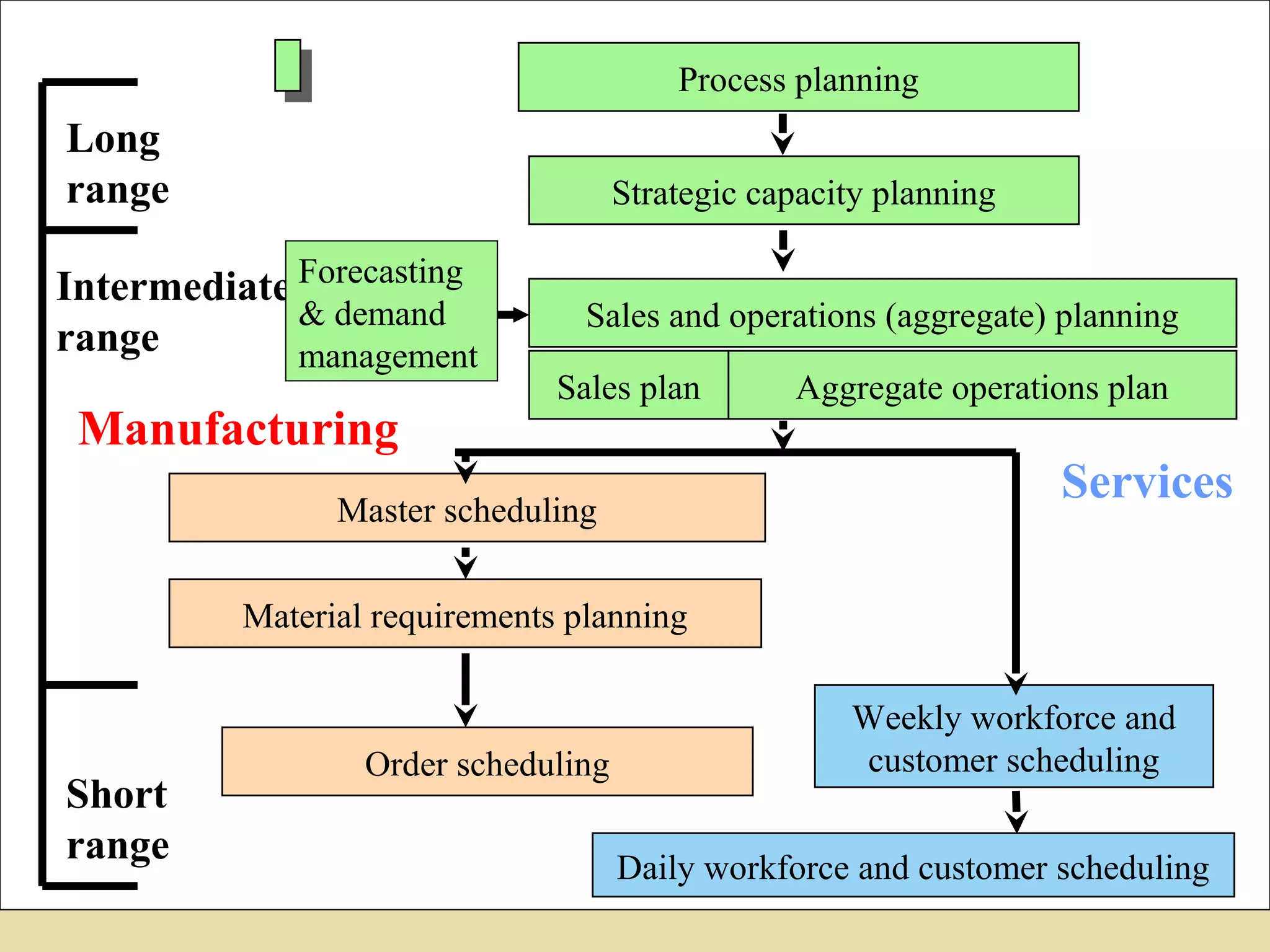
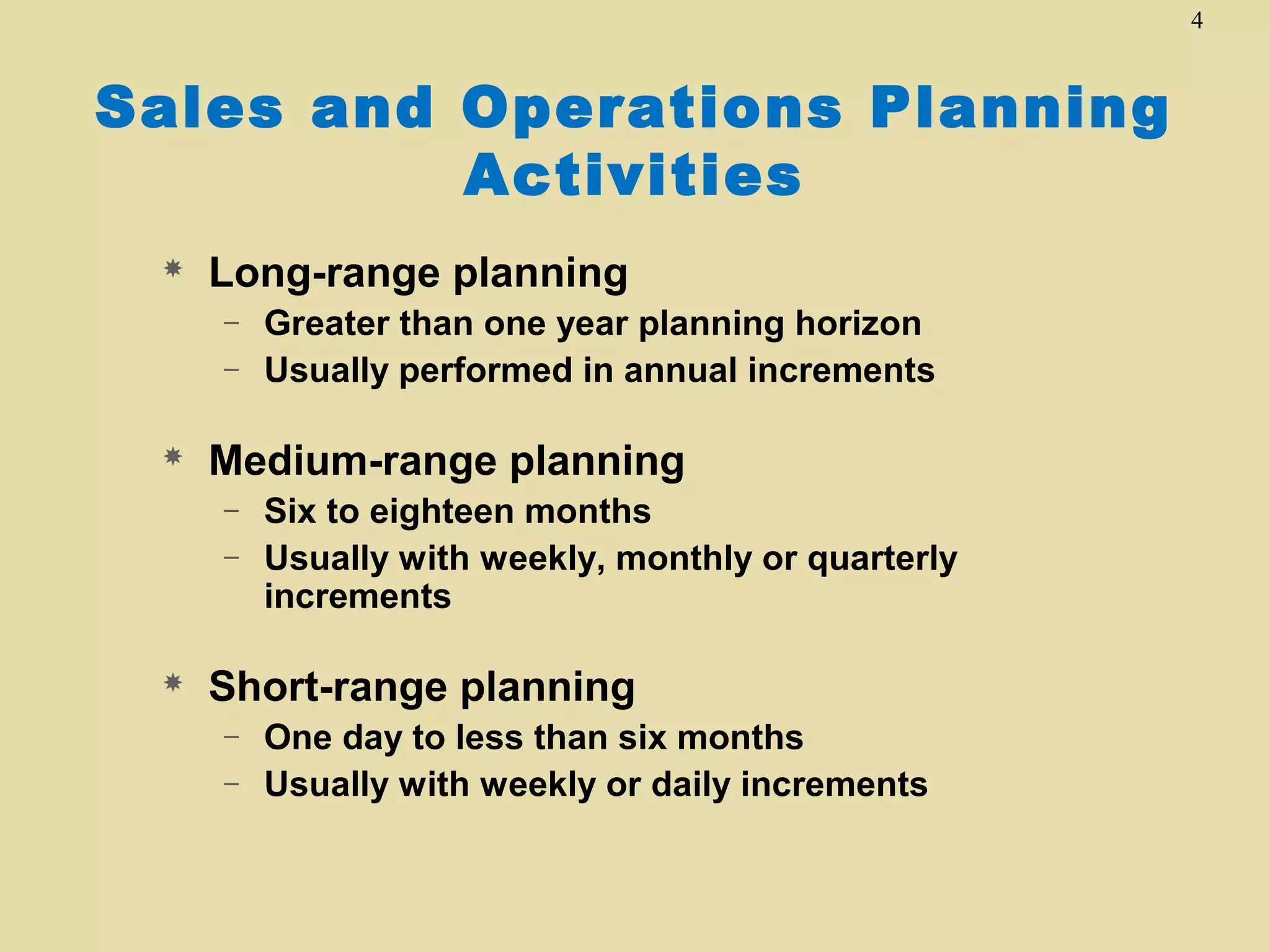
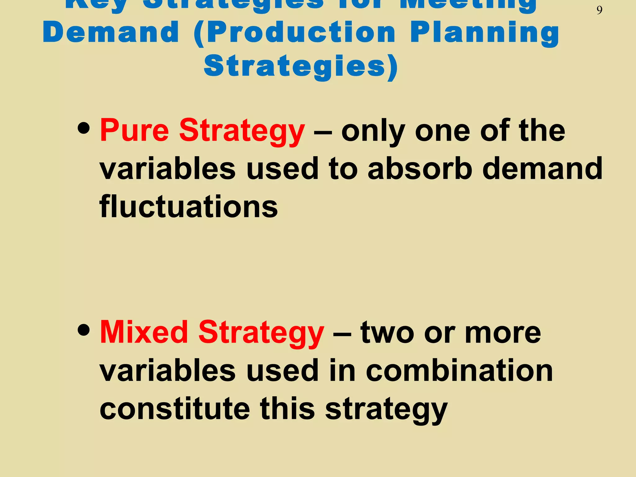
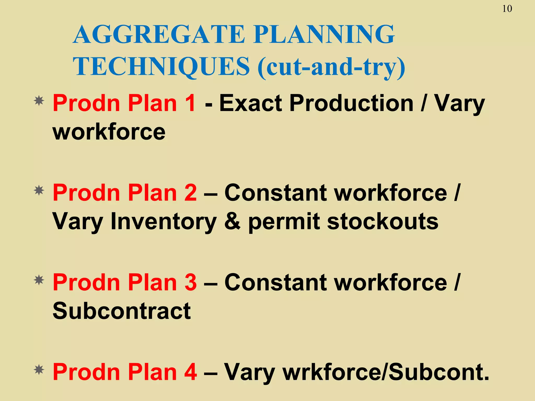
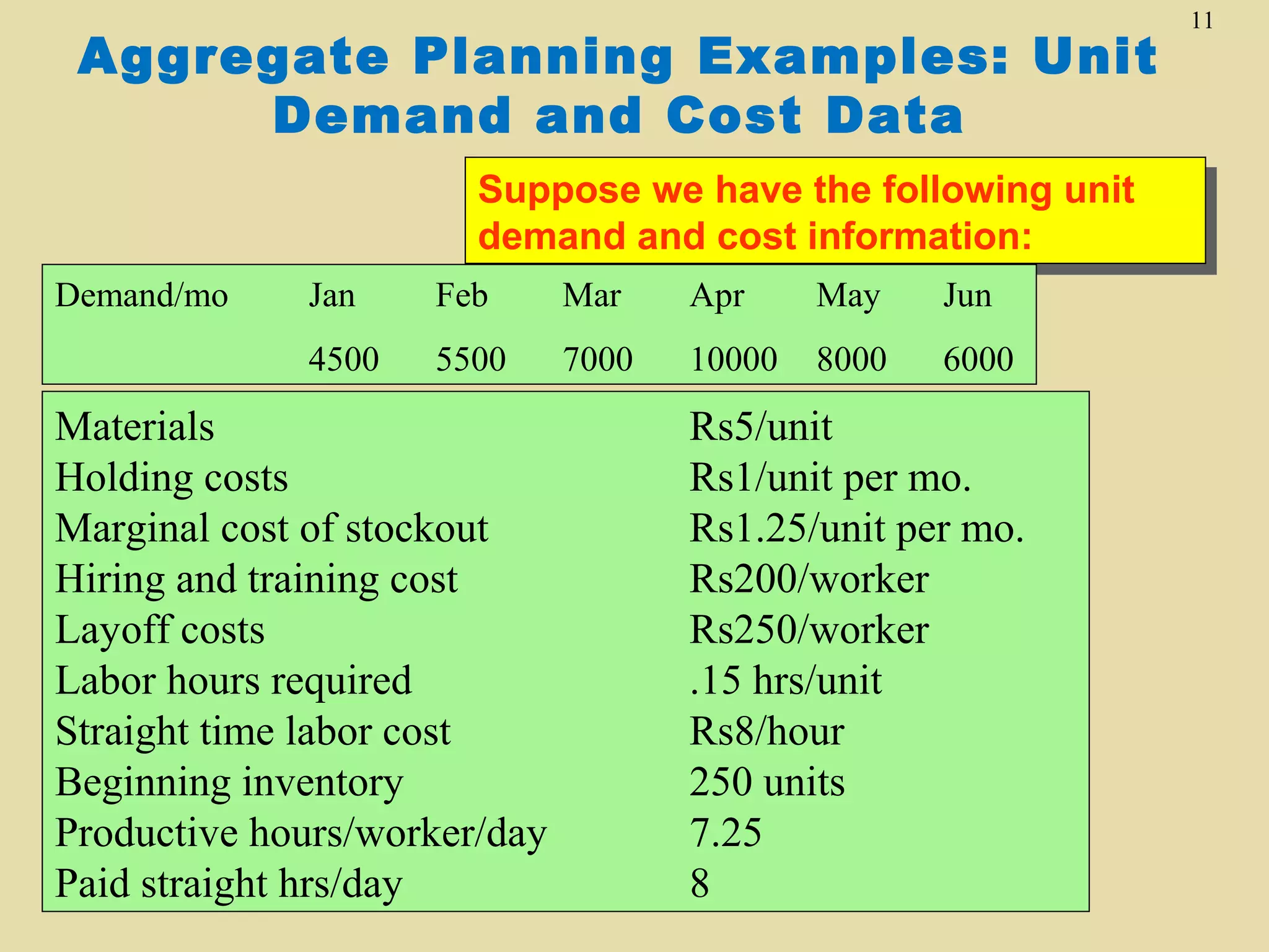
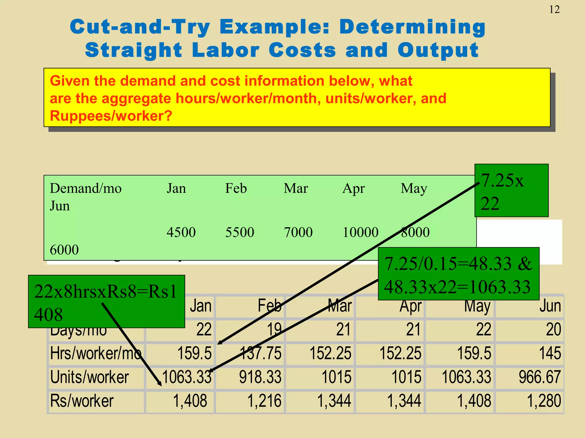
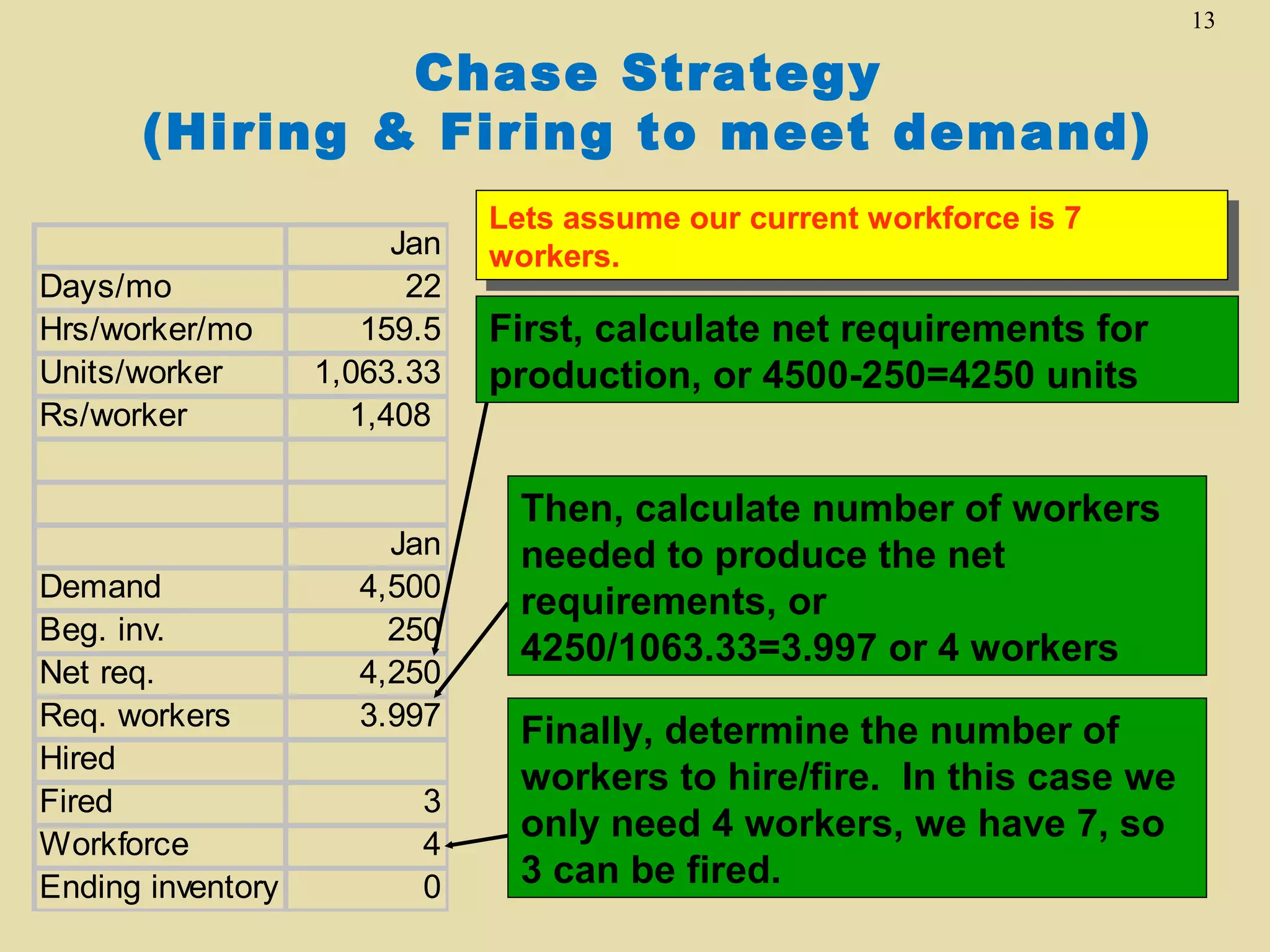
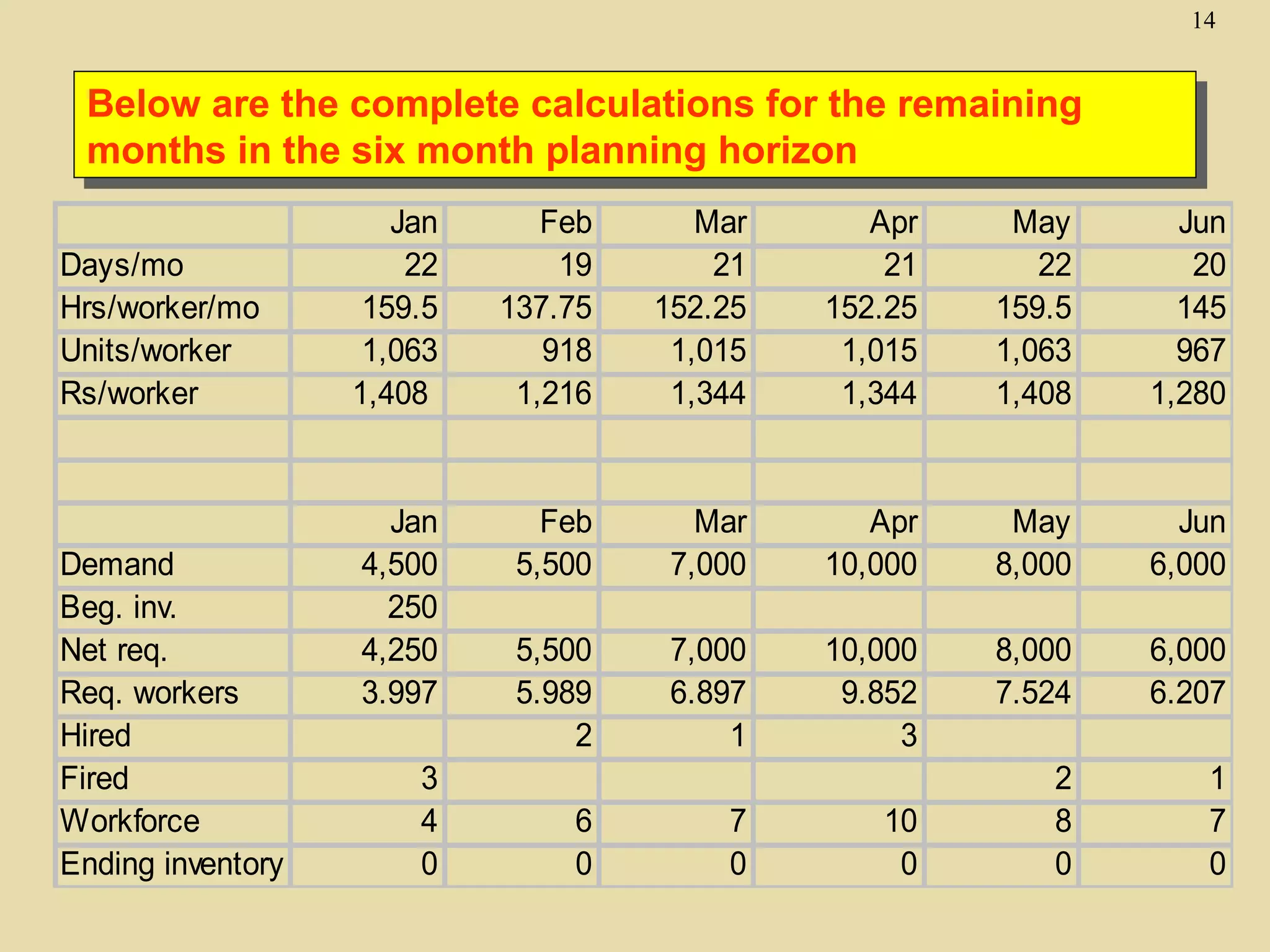
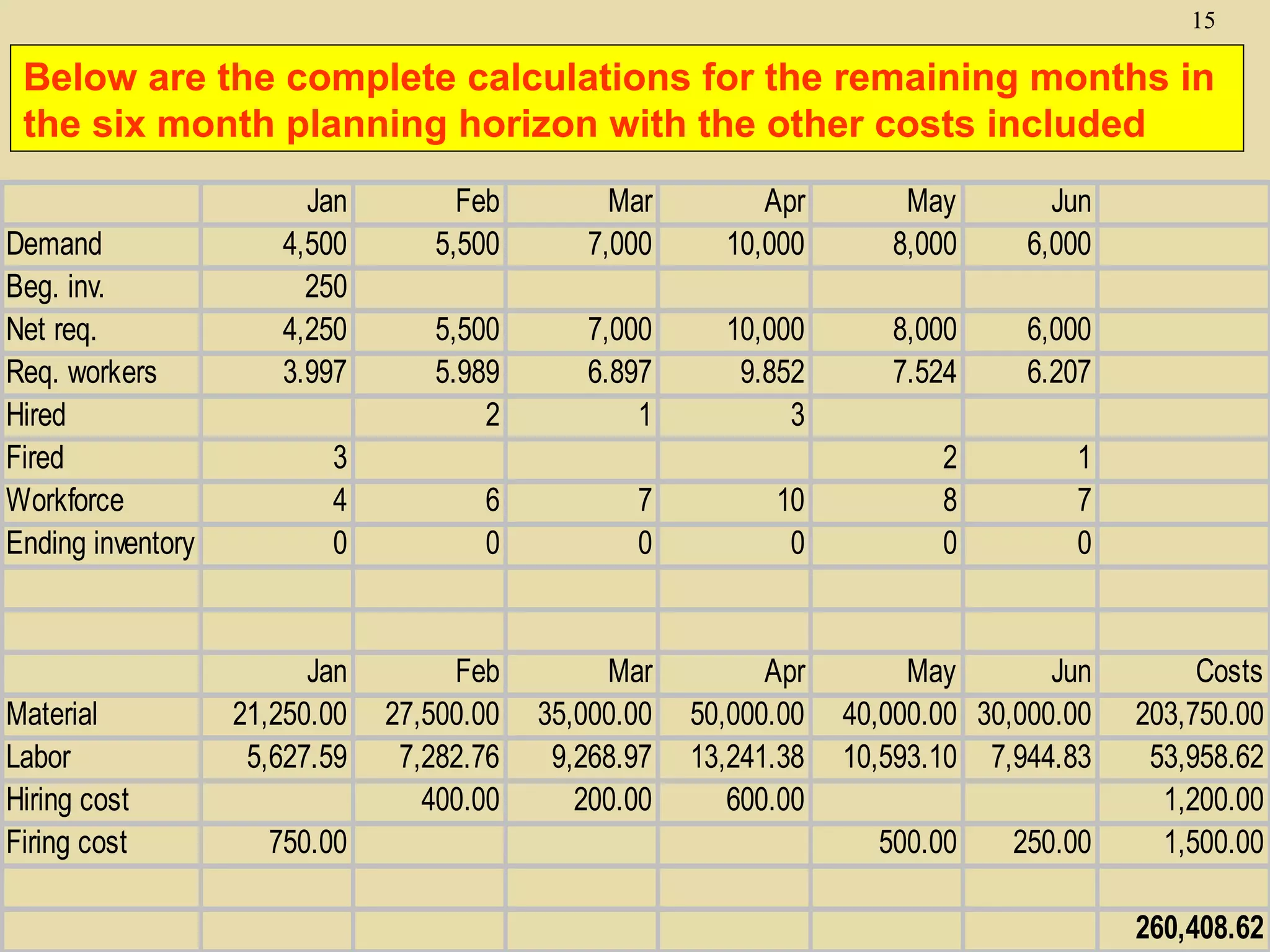
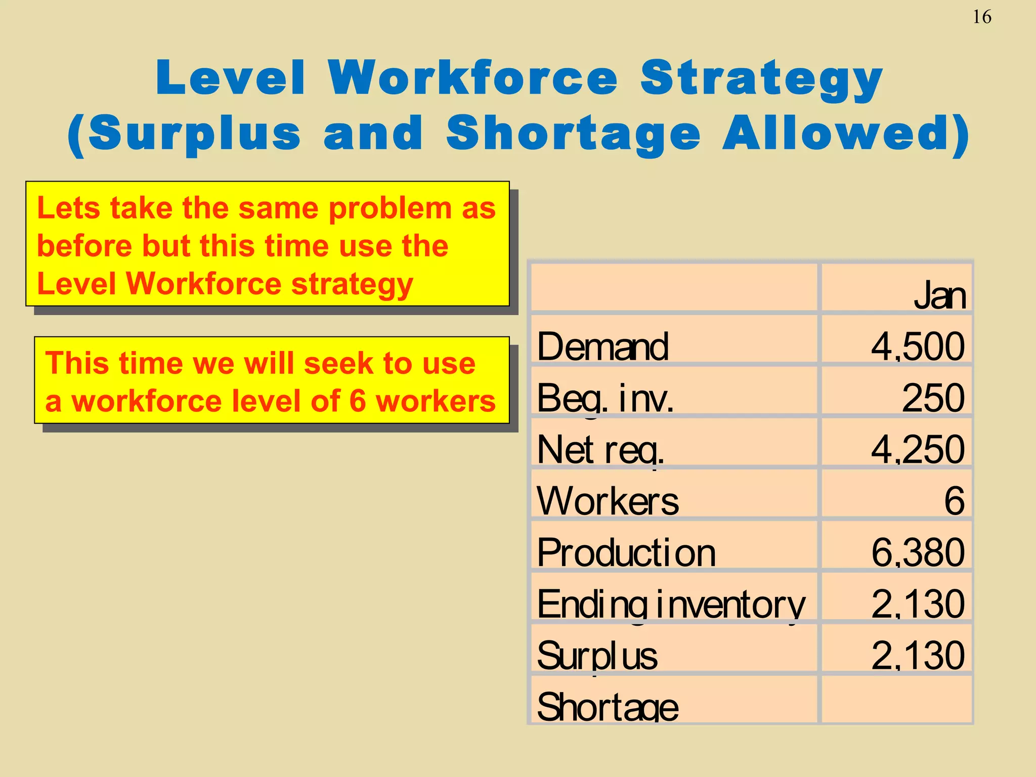
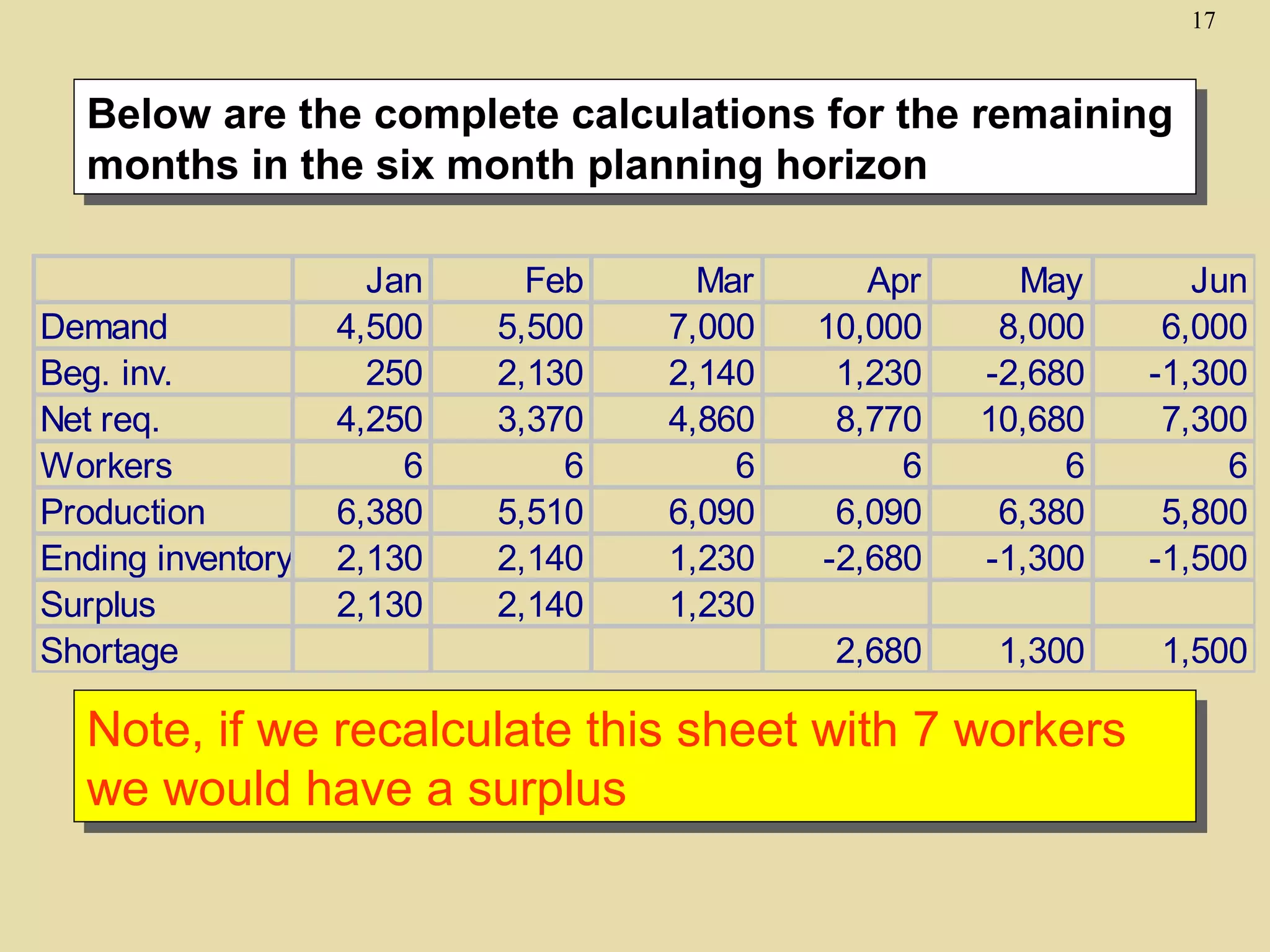
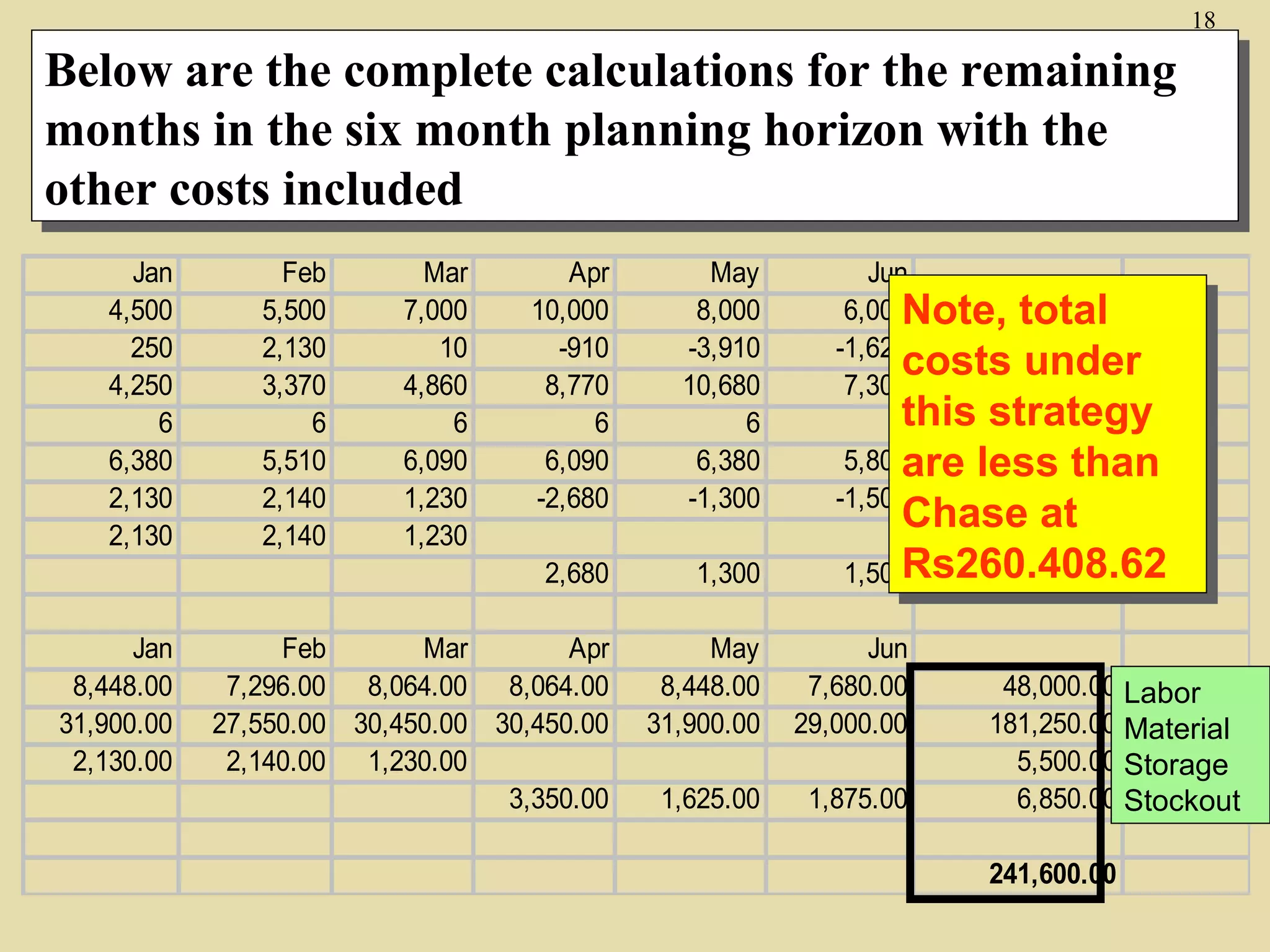
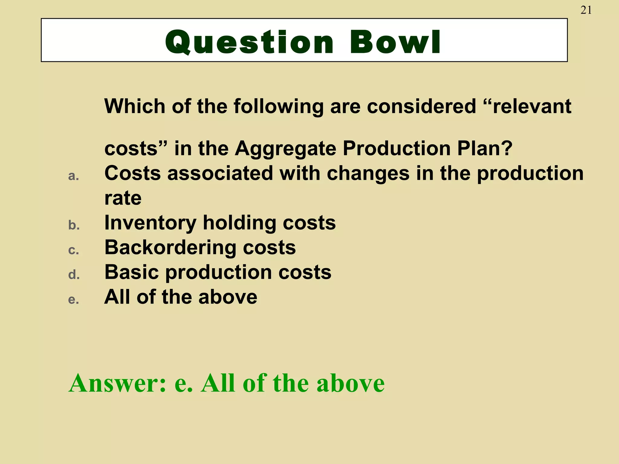
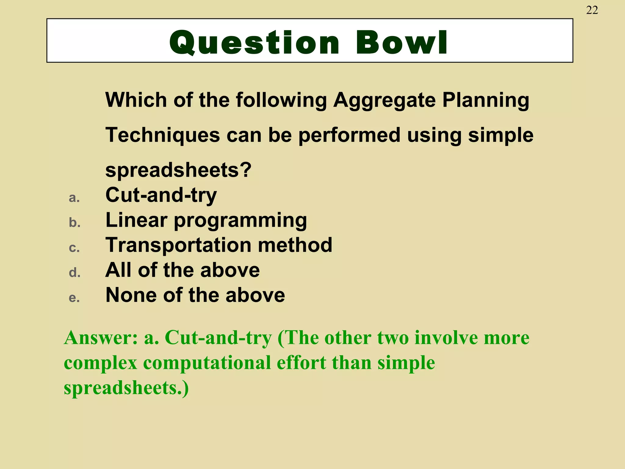
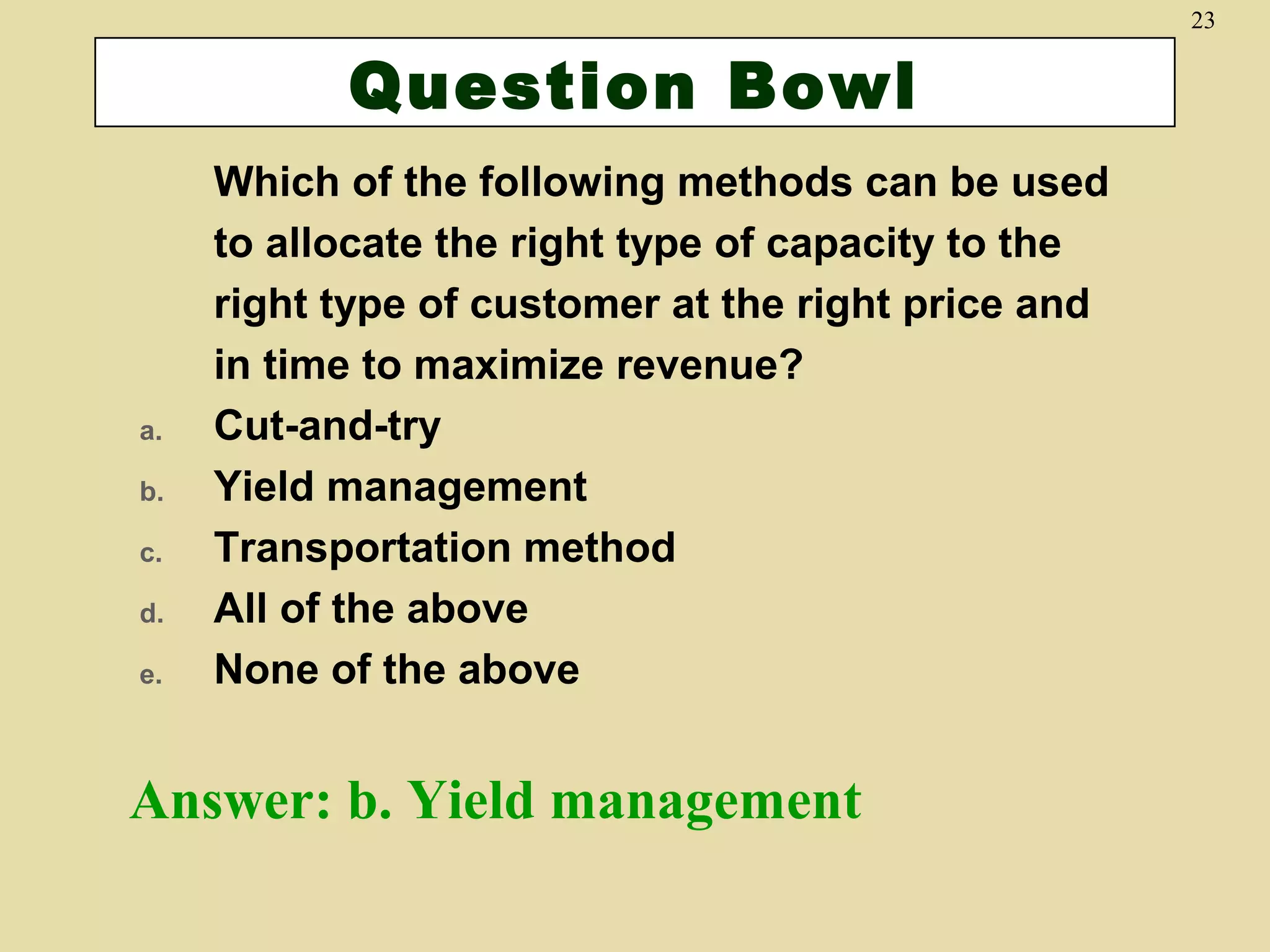
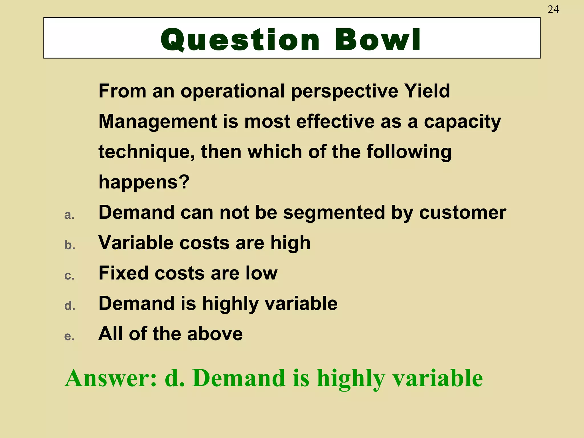
1

Aggregate Sales and Operations Planning
2

OBJECTIVES


Sales and Operations Planning



The Aggregate Operations Plan



Examples: Chase and Level
strategies
3

Process planning

Long
range

Strategic capacity planning

Intermediate Forecasting
& demand
range
management

Manufacturing

Sales and operations (aggregate) planning
Sales plan

Aggregate operations plan

Services

Master scheduling
Material requirements planning

Short
range

Order scheduling

Weekly workforce and
customer scheduling
Daily workforce and customer scheduling
4

Sales and Operations Planning
Activities


Long-range planning
–
–



Medium-range planning
–
–



Greater than one year planning horizon
Usually performed in annual increments

Six to eighteen months
Usually with weekly, monthly or quarterly
increments

Short-range planning
–
–

One day to less than six months
Usually with weekly or daily increments
The Aggregate Operations
Plan

• Main purpose: Specify the optimal
combination of

•

production rate (units completed per unit
of time)

•
•

workforce level (number of workers)
inventory on hand (inventory carried from
previous period)

• Product group or broad category
(Aggregation)
• This planning is done over an intermediaterange planning period of 3 to18 months

5
Balancing Aggregate Demand
and Aggregate Production
Capacity
Suppose the figure to
the right represents
forecast demand in
forecast demand in
units
units
Now suppose this
Now suppose this
lower figure represents
the aggregate capacity
of the company to
of the company to
meet demand
meet demand

10000

10000

8000

8000
6000

7000
6000

5500
4500

4000
2000
0
Jan

Feb

Mar
9000

10000

Apr

May

Jun

8000

8000

What we want to do is
balance out the
balance out the
production rate,
production rate,
workforce levels, and
inventory to make
inventory to make
these figures match up

6000

6000
4500

4000

Jan

Feb

4000

4000
2000
0
Mar

Apr

May

Jun

6
7

Required Inputs to the Production
Planning System
Competitors’
behavior
External
capacity

Current
physical
capacity

Raw material
availability

Planning
for
production

Current
workforce

Inventory
levels

Market
demand

External
to firm

Economic
conditions

Activities
required
for
production

Internal
to firm
Key Strategies for Meeting
Demand (Production Planning
Strategies)

• Chase Strategy
• Stable workforce – variable work
hours

• Level Strategy

8
Key Strategies for Meeting
Demand (Production Planning
Strategies)

• Pure Strategy – only one of the

9

variables used to absorb demand
fluctuations

• Mixed Strategy – two or more

variables used in combination
constitute this strategy
10

AGGREGATE PLANNING
TECHNIQUES (cut-and-try)


Prodn Plan 1 - Exact Production / Vary
workforce



Prodn Plan 2 – Constant workforce /
Vary Inventory & permit stockouts



Prodn Plan 3 – Constant workforce /
Subcontract



Prodn Plan 4 – Vary wrkforce/Subcont.
Aggregate Planning Examples: Unit
Demand and Cost Data
Suppose we have the following unit
demand and cost information:
Demand/mo

Jan

Feb

Mar

Apr

May

Jun

4500

5500

7000

10000

8000

6000

Materials
Holding costs
Marginal cost of stockout
Hiring and training cost
Layoff costs
Labor hours required
Straight time labor cost
Beginning inventory
Productive hours/worker/day
Paid straight hrs/day

Rs5/unit
Rs1/unit per mo.
Rs1.25/unit per mo.
Rs200/worker
Rs250/worker
.15 hrs/unit
Rs8/hour
250 units
7.25
8

11
12

Cut-and-Try Example: Determining
Straight Labor Costs and Output
Given the demand and cost information below, what
are the aggregate hours/worker/month, units/worker, and
Ruppees/worker?
Ruppees/worker?

Demand/mo
Jun

Jan

Feb

4500
5500
Productive hours/worker/day
6000 straight hrs/day
Paid

22x8hrsxRs8=Rs1
Jan
408
Days/mo
Hrs/worker/mo
Units/worker
Rs/worker

22
159.5
1063.33
1,408

Feb
19
137.75
918.33
1,216

Mar

Apr

May

7000
7.25

10000

7.25x
22

8000

8

Mar
21
152.25
1015
1,344

7.25/0.15=48.33 &
48.33x22=1063.33

Apr
21
152.25
1015
1,344

May
22
159.5
1063.33
1,408

Jun
20
145
966.67
1,280
13

Chase Strategy
(Hiring & Firing to meet demand)
Days/mo
Hrs/worker/mo
Units/worker
Rs/worker

Demand
Beg. inv.
Net req.
Req. workers
Hired
Fired
Workforce
Ending inventory

Jan
22
159.5
1,063.33
1,408

Jan
4,500
250
4,250
3.997
3
4
0

Lets assume our current workforce is 7
workers.
workers.

First, calculate net requirements for
production, or 4500-250=4250 units
Then, calculate number of workers
needed to produce the net
requirements, or
4250/1063.33=3.997 or 4 workers
Finally, determine the number of
workers to hire/fire. In this case we
only need 4 workers, we have 7, so
3 can be fired.
14

Below are the complete calculations for the remaining
months in the six month planning horizon
Days/mo
Hrs/worker/mo
Units/worker
Rs/worker

Demand
Beg. inv.
Net req.
Req. workers
Hired
Fired
Workforce
Ending inventory

Jan
22
159.5
1,063
1,408

Feb
19
137.75
918
1,216

Mar
21
152.25
1,015
1,344

Apr
21
152.25
1,015
1,344

May
22
159.5
1,063
1,408

Jun
20
145
967
1,280

Jan
4,500
250
4,250
3.997

Feb
5,500

Mar
7,000

Apr
10,000

May
8,000

Jun
6,000

5,500
5.989
2

7,000
6.897
1

10,000
9.852
3

8,000
7.524

6,000
6.207

2
8
0

1
7
0

3
4
0

6
0

7
0

10
0
15

Below are the complete calculations for the remaining months in
the six month planning horizon with the other costs included
Demand
Beg. inv.
Net req.
Req. workers
Hired
Fired
Workforce
Ending inventory

Material
Labor
Hiring cost
Firing cost

Jan
4,500
250
4,250
3.997
3
4
0

Jan
21,250.00
5,627.59
750.00

Feb
5,500

Mar
7,000

Apr
10,000

May
8,000

Jun
6,000

5,500
5.989
2

7,000
6.897
1

10,000
9.852
3

8,000
7.524

6,000
6.207

2
8
0

1
7
0

6
0

7
0

10
0

Feb
27,500.00
7,282.76
400.00

Mar
35,000.00
9,268.97
200.00

Apr
50,000.00
13,241.38
600.00

May
Jun
40,000.00 30,000.00
10,593.10 7,944.83
500.00

250.00

Costs
203,750.00
53,958.62
1,200.00
1,500.00
260,408.62
16

Level Workforce Strategy
(Surplus and Shortage Allowed)
Lets take the same problem as
before but this time use the
Level Workforce strategy
This time we will seek to use
a workforce level of 6 workers

Demand
Beg. inv.
Net req.
Workers
Production
Ending inventory
Surplus
Shortage

Jan
4,500
250
4,250
6
6,380
2,130
2,130
17

Below are the complete calculations for the remaining
months in the six month planning horizon

Demand
Beg. inv.
Net req.
Workers
Production
Ending inventory
Surplus
Shortage

Jan
4,500
250
4,250
6
6,380
2,130
2,130

Feb
5,500
2,130
3,370
6
5,510
2,140
2,140

Mar
7,000
2,140
4,860
6
6,090
1,230
1,230

Apr
10,000
1,230
8,770
6
6,090
-2,680

May
8,000
-2,680
10,680
6
6,380
-1,300

Jun
6,000
-1,300
7,300
6
5,800
-1,500

2,680

1,300

1,500

Note, if we recalculate this sheet with 7 workers
we would have a surplus
18

Below are the complete calculations for the remaining
months in the six month planning horizon with the
other costs included
Jan
4,500
250
4,250
6
6,380
2,130
2,130

Apr
10,000
-910
8,770
6
6,090
-2,680

May
8,000
-3,910
10,680
6
6,380
-1,300

2,680
Jan
8,448.00
31,900.00
2,130.00

Feb
5,500
2,130
3,370
6
5,510
2,140
2,140

Mar
7,000
10
4,860
6
6,090
1,230
1,230

Jun
6,000
Note, total
Note, total
-1,620
costs under
7,300 costs under
this strategy
6 this strategy
5,800
are less than
are less than
-1,500

1,300

Feb
Mar
Apr
7,296.00 8,064.00 8,064.00
27,550.00 30,450.00 30,450.00
2,140.00 1,230.00
3,350.00

May
8,448.00
31,900.00

Jun
7,680.00
29,000.00

1,625.00

1,875.00

Chase at
Chase at
Rs260.408.62
1,500 Rs260.408.62
48,000.00 Labor
181,250.00 Material
5,500.00 Storage
6,850.00 Stockout
241,600.00
19

Question Bowl

a.
b.
c.
d.
e.

Sales and Operations Planning activities
are usually conducted during which
planning time horizon?
Long-range
Intermediate-range
Short-range
Really short-range
None of the above

Answer: b. Intermediate-range (i.e., 6 to
18 months)
20

Question Bowl

a.
b.
c.
d.
e.

Which of the following are Production Planning
Strategies can involve trade-offs among the
workforce size, work hours, inventory, and
backlogs?
Chase strategy
Stable workforce-variable work hours
Level strategy
All of the above
None of the above

Answer: d. All of the above
21

Question Bowl
Which of the following are considered “relevant
a.

b.
c.
d.
e.

costs” in the Aggregate Production Plan?
Costs associated with changes in the production
rate
Inventory holding costs
Backordering costs
Basic production costs
All of the above

Answer: e. All of the above
22

Question Bowl
Which of the following Aggregate Planning
Techniques can be performed using simple
a.
b.
c.
d.
e.

spreadsheets?
Cut-and-try
Linear programming
Transportation method
All of the above
None of the above

Answer: a. Cut-and-try (The other two involve more
complex computational effort than simple
spreadsheets.)
23

Question Bowl

a.
b.
c.
d.
e.

Which of the following methods can be used
to allocate the right type of capacity to the
right type of customer at the right price and
in time to maximize revenue?
Cut-and-try
Yield management
Transportation method
All of the above
None of the above

Answer: b. Yield management
24

Question Bowl
From an operational perspective Yield
Management is most effective as a capacity
technique, then which of the following
happens?
a.

Demand can not be segmented by customer

b.

Variable costs are high

c.

Fixed costs are low

d.

Demand is highly variable

e.

All of the above

Answer: d. Demand is highly variable

Ch14 aggt.sales & op.planning

  • 1.
    1 Aggregate Sales andOperations Planning
  • 2.
    2 OBJECTIVES  Sales and OperationsPlanning  The Aggregate Operations Plan  Examples: Chase and Level strategies
  • 3.
    3 Process planning Long range Strategic capacityplanning Intermediate Forecasting & demand range management Manufacturing Sales and operations (aggregate) planning Sales plan Aggregate operations plan Services Master scheduling Material requirements planning Short range Order scheduling Weekly workforce and customer scheduling Daily workforce and customer scheduling
  • 4.
    4 Sales and OperationsPlanning Activities  Long-range planning – –  Medium-range planning – –  Greater than one year planning horizon Usually performed in annual increments Six to eighteen months Usually with weekly, monthly or quarterly increments Short-range planning – – One day to less than six months Usually with weekly or daily increments
  • 5.
    The Aggregate Operations Plan •Main purpose: Specify the optimal combination of • production rate (units completed per unit of time) • • workforce level (number of workers) inventory on hand (inventory carried from previous period) • Product group or broad category (Aggregation) • This planning is done over an intermediaterange planning period of 3 to18 months 5
  • 6.
    Balancing Aggregate Demand andAggregate Production Capacity Suppose the figure to Suppose the figure to the right represents the right represents forecast demand in forecast demand in units units Now suppose this Now suppose this lower figure represents lower figure represents the aggregate capacity the aggregate capacity of the company to of the company to meet demand meet demand 10000 10000 8000 8000 6000 7000 6000 5500 4500 4000 2000 0 Jan Feb Mar 9000 10000 Apr May Jun 8000 8000 What we want to do is What we want to do is balance out the balance out the production rate, production rate, workforce levels, and workforce levels, and inventory to make inventory to make these figures match up these figures match up 6000 6000 4500 4000 Jan Feb 4000 4000 2000 0 Mar Apr May Jun 6
  • 7.
    7 Required Inputs tothe Production Planning System Competitors’ behavior External capacity Current physical capacity Raw material availability Planning for production Current workforce Inventory levels Market demand External to firm Economic conditions Activities required for production Internal to firm
  • 8.
    Key Strategies forMeeting Demand (Production Planning Strategies) • Chase Strategy • Stable workforce – variable work hours • Level Strategy 8
  • 9.
    Key Strategies forMeeting Demand (Production Planning Strategies) • Pure Strategy – only one of the 9 variables used to absorb demand fluctuations • Mixed Strategy – two or more variables used in combination constitute this strategy
  • 10.
    10 AGGREGATE PLANNING TECHNIQUES (cut-and-try)  ProdnPlan 1 - Exact Production / Vary workforce  Prodn Plan 2 – Constant workforce / Vary Inventory & permit stockouts  Prodn Plan 3 – Constant workforce / Subcontract  Prodn Plan 4 – Vary wrkforce/Subcont.
  • 11.
    Aggregate Planning Examples:Unit Demand and Cost Data Suppose we have the following unit Suppose we have the following unit demand and cost information: demand and cost information: Demand/mo Jan Feb Mar Apr May Jun 4500 5500 7000 10000 8000 6000 Materials Holding costs Marginal cost of stockout Hiring and training cost Layoff costs Labor hours required Straight time labor cost Beginning inventory Productive hours/worker/day Paid straight hrs/day Rs5/unit Rs1/unit per mo. Rs1.25/unit per mo. Rs200/worker Rs250/worker .15 hrs/unit Rs8/hour 250 units 7.25 8 11
  • 12.
    12 Cut-and-Try Example: Determining StraightLabor Costs and Output Given the demand and cost information below, what Given the demand and cost information below, what are the aggregate hours/worker/month, units/worker, and are the aggregate hours/worker/month, units/worker, and Ruppees/worker? Ruppees/worker? Demand/mo Jun Jan Feb 4500 5500 Productive hours/worker/day 6000 straight hrs/day Paid 22x8hrsxRs8=Rs1 Jan 408 Days/mo Hrs/worker/mo Units/worker Rs/worker 22 159.5 1063.33 1,408 Feb 19 137.75 918.33 1,216 Mar Apr May 7000 7.25 10000 7.25x 22 8000 8 Mar 21 152.25 1015 1,344 7.25/0.15=48.33 & 48.33x22=1063.33 Apr 21 152.25 1015 1,344 May 22 159.5 1063.33 1,408 Jun 20 145 966.67 1,280
  • 13.
    13 Chase Strategy (Hiring &Firing to meet demand) Days/mo Hrs/worker/mo Units/worker Rs/worker Demand Beg. inv. Net req. Req. workers Hired Fired Workforce Ending inventory Jan 22 159.5 1,063.33 1,408 Jan 4,500 250 4,250 3.997 3 4 0 Lets assume our current workforce is 7 Lets assume our current workforce is 7 workers. workers. First, calculate net requirements for production, or 4500-250=4250 units Then, calculate number of workers needed to produce the net requirements, or 4250/1063.33=3.997 or 4 workers Finally, determine the number of workers to hire/fire. In this case we only need 4 workers, we have 7, so 3 can be fired.
  • 14.
    14 Below are thecomplete calculations for the remaining Below are the complete calculations for the remaining months in the six month planning horizon months in the six month planning horizon Days/mo Hrs/worker/mo Units/worker Rs/worker Demand Beg. inv. Net req. Req. workers Hired Fired Workforce Ending inventory Jan 22 159.5 1,063 1,408 Feb 19 137.75 918 1,216 Mar 21 152.25 1,015 1,344 Apr 21 152.25 1,015 1,344 May 22 159.5 1,063 1,408 Jun 20 145 967 1,280 Jan 4,500 250 4,250 3.997 Feb 5,500 Mar 7,000 Apr 10,000 May 8,000 Jun 6,000 5,500 5.989 2 7,000 6.897 1 10,000 9.852 3 8,000 7.524 6,000 6.207 2 8 0 1 7 0 3 4 0 6 0 7 0 10 0
  • 15.
    15 Below are thecomplete calculations for the remaining months in the six month planning horizon with the other costs included Demand Beg. inv. Net req. Req. workers Hired Fired Workforce Ending inventory Material Labor Hiring cost Firing cost Jan 4,500 250 4,250 3.997 3 4 0 Jan 21,250.00 5,627.59 750.00 Feb 5,500 Mar 7,000 Apr 10,000 May 8,000 Jun 6,000 5,500 5.989 2 7,000 6.897 1 10,000 9.852 3 8,000 7.524 6,000 6.207 2 8 0 1 7 0 6 0 7 0 10 0 Feb 27,500.00 7,282.76 400.00 Mar 35,000.00 9,268.97 200.00 Apr 50,000.00 13,241.38 600.00 May Jun 40,000.00 30,000.00 10,593.10 7,944.83 500.00 250.00 Costs 203,750.00 53,958.62 1,200.00 1,500.00 260,408.62
  • 16.
    16 Level Workforce Strategy (Surplusand Shortage Allowed) Lets take the same problem as Lets take the same problem as before but this time use the before but this time use the Level Workforce strategy Level Workforce strategy This time we will seek to use This time we will seek to use a workforce level of 6 workers a workforce level of 6 workers Demand Beg. inv. Net req. Workers Production Ending inventory Surplus Shortage Jan 4,500 250 4,250 6 6,380 2,130 2,130
  • 17.
    17 Below are thecomplete calculations for the remaining Below are the complete calculations for the remaining months in the six month planning horizon months in the six month planning horizon Demand Beg. inv. Net req. Workers Production Ending inventory Surplus Shortage Jan 4,500 250 4,250 6 6,380 2,130 2,130 Feb 5,500 2,130 3,370 6 5,510 2,140 2,140 Mar 7,000 2,140 4,860 6 6,090 1,230 1,230 Apr 10,000 1,230 8,770 6 6,090 -2,680 May 8,000 -2,680 10,680 6 6,380 -1,300 Jun 6,000 -1,300 7,300 6 5,800 -1,500 2,680 1,300 1,500 Note, if we recalculate this sheet with 7 workers Note, if we recalculate this sheet with 7 workers we would have a surplus we would have a surplus
  • 18.
    18 Below are thecomplete calculations for the remaining Below are the complete calculations for the remaining months in the six month planning horizon with the months in the six month planning horizon with the other costs included other costs included Jan 4,500 250 4,250 6 6,380 2,130 2,130 Apr 10,000 -910 8,770 6 6,090 -2,680 May 8,000 -3,910 10,680 6 6,380 -1,300 2,680 Jan 8,448.00 31,900.00 2,130.00 Feb 5,500 2,130 3,370 6 5,510 2,140 2,140 Mar 7,000 10 4,860 6 6,090 1,230 1,230 Jun 6,000 Note, total Note, total -1,620 costs under 7,300 costs under this strategy 6 this strategy 5,800 are less than are less than -1,500 1,300 Feb Mar Apr 7,296.00 8,064.00 8,064.00 27,550.00 30,450.00 30,450.00 2,140.00 1,230.00 3,350.00 May 8,448.00 31,900.00 Jun 7,680.00 29,000.00 1,625.00 1,875.00 Chase at Chase at Rs260.408.62 1,500 Rs260.408.62 48,000.00 Labor 181,250.00 Material 5,500.00 Storage 6,850.00 Stockout 241,600.00
  • 19.
    19 Question Bowl a. b. c. d. e. Sales andOperations Planning activities are usually conducted during which planning time horizon? Long-range Intermediate-range Short-range Really short-range None of the above Answer: b. Intermediate-range (i.e., 6 to 18 months)
  • 20.
    20 Question Bowl a. b. c. d. e. Which ofthe following are Production Planning Strategies can involve trade-offs among the workforce size, work hours, inventory, and backlogs? Chase strategy Stable workforce-variable work hours Level strategy All of the above None of the above Answer: d. All of the above
  • 21.
    21 Question Bowl Which ofthe following are considered “relevant a. b. c. d. e. costs” in the Aggregate Production Plan? Costs associated with changes in the production rate Inventory holding costs Backordering costs Basic production costs All of the above Answer: e. All of the above
  • 22.
    22 Question Bowl Which ofthe following Aggregate Planning Techniques can be performed using simple a. b. c. d. e. spreadsheets? Cut-and-try Linear programming Transportation method All of the above None of the above Answer: a. Cut-and-try (The other two involve more complex computational effort than simple spreadsheets.)
  • 23.
    23 Question Bowl a. b. c. d. e. Which ofthe following methods can be used to allocate the right type of capacity to the right type of customer at the right price and in time to maximize revenue? Cut-and-try Yield management Transportation method All of the above None of the above Answer: b. Yield management
  • 24.
    24 Question Bowl From anoperational perspective Yield Management is most effective as a capacity technique, then which of the following happens? a. Demand can not be segmented by customer b. Variable costs are high c. Fixed costs are low d. Demand is highly variable e. All of the above Answer: d. Demand is highly variable