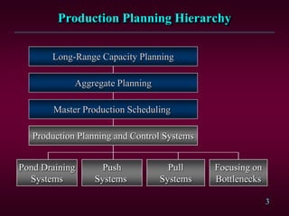
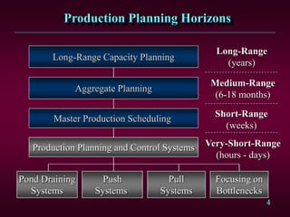
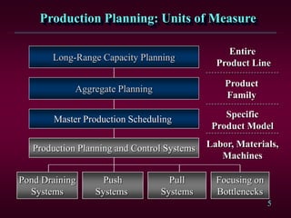
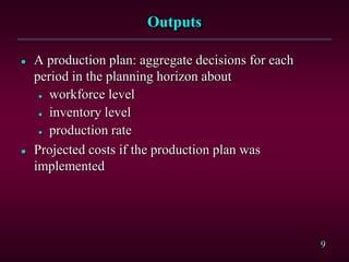
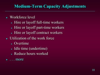
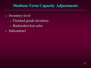
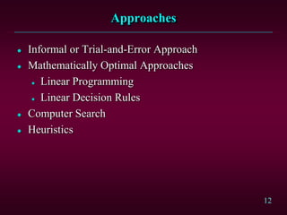
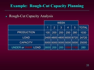
This document discusses production planning concepts including the production planning hierarchy, aggregate planning, master production scheduling, and types of production planning and control systems. It provides information on aggregate planning inputs and outputs, approaches to aggregate planning, and examples of developing a master production schedule and rough-cut capacity plan. It also describes different types of production planning systems such as pond draining, push, pull, and bottleneck-focused systems.

1. 1
Chapter 13
Production Planning

2. 2
Overview
 Production-Planning Hierarchy
 Aggregate Planning
 Master Production Scheduling
 Types of Production-Planning and Control Systems
 Wrap-Up: What World-Class Companies Do

3. 3
Production Planning Hierarchy
Master Production Scheduling
Production Planning and Control Systems
Pond Draining
Systems
Aggregate Planning
Push
Systems
Pull
Systems
Focusing on
Bottlenecks
Long-Range Capacity Planning

4. 4
Production Planning Horizons
Master Production Scheduling
Production Planning and Control Systems
Pond Draining
Systems
Aggregate Planning
Push
Systems
Pull
Systems
Focusing on
Bottlenecks
Long-Range Capacity Planning
Long-Range
(years)
Medium-Range
(6-18 months)
Short-Range
(weeks)
Very-Short-Range
(hours - days)

5. 5
Production Planning: Units of Measure
Master Production Scheduling
Production Planning and Control Systems
Pond Draining
Systems
Aggregate Planning
Push
Systems
Pull
Systems
Focusing on
Bottlenecks
Long-Range Capacity Planning
Entire
Product Line
Product
Family
Specific
Product Model
Labor, Materials,
Machines

6. 6
Aggregate Planning

7. 7
Why Aggregate Planning Is Necessary
 Fully load facilities and minimize overloading and
underloading
 Make sure enough capacity available to satisfy
expected demand
 Plan for the orderly and systematic change of
production capacity to meet the peaks and valleys of
expected customer demand
 Get the most output for the amount of resources
available

8. 8
Inputs
 A forecast of aggregate demand covering the selected
planning horizon (6-18 months)
 The alternative means available to adjust short- to
medium-term capacity, to what extent each
alternative could impact capacity and the related costs
 The current status of the system in terms of
workforce level, inventory level and production rate

9. 9
Outputs
 A production plan: aggregate decisions for each
period in the planning horizon about
 workforce level
 inventory level
 production rate
 Projected costs if the production plan was
implemented

10. 10
Medium-Term Capacity Adjustments
 Workforce level
 Hire or layoff full-time workers
 Hire or layoff part-time workers
 Hire or layoff contract workers
 Utilization of the work force
 Overtime
 Idle time (undertime)
 Reduce hours worked
 . . . more

11. 11
Medium-Term Capacity Adjustments
 Inventory level
 Finished goods inventory
 Backorders/lost sales
 Subcontract

12. 12
Approaches
 Informal or Trial-and-Error Approach
 Mathematically Optimal Approaches
 Linear Programming
 Linear Decision Rules
 Computer Search
 Heuristics

13. 13
Pure Strategies for the Informal Approach
 Matching Demand
 Level Capacity
 Buffering with inventory
 Buffering with backlog
 Buffering with overtime or subcontracting

14. 14
Matching Demand Strategy
 Capacity (Production) in each time period is varied to
exactly match the forecasted aggregate demand in
that time period
 Capacity is varied by changing the workforce level
 Finished-goods inventories are minimal
 Labor and materials costs tend to be high due to the
frequent changes

15. 15
Developing and Evaluating
the Matching Production Plan
 Production rate is dictated by the forecasted aggregate
demand
 Convert the forecasted aggregate demand into the
required workforce level using production time
information
 The primary costs of this strategy are the costs of
changing workforce levels from period to period, i.e.,
hirings and layoffs

16. 16
Level Capacity Strategy
 Capacity (production rate) is held level (constant)
over the planning horizon
 The difference between the constant production rate
and the demand rate is made up (buffered) by
inventory, backlog, overtime, part-time labor and/or
subcontracting

17. 17
Developing and Evaluating
the Level Production Plan
 Assume that the amount produced each period is
constant, no hirings or layoffs
 The gap between the amount planned to be produced
and the forecasted demand is filled with either
inventory or backorders, i.e., no overtime, no idle
time, no subcontracting
 . . . more

18. 18
Developing and Evaluating
the Level Production Plan
 The primary costs of this strategy are inventory
carrying and backlogging costs
 Period-ending inventories or backlogs are determined
using the inventory balance equation:
EIt = EIt-1 + (Pt - Dt )

19. 19
Aggregate Plans for Services
 For standardized services, aggregate planning may be
simpler than in systems that produce products
 For customized services,
 there may be difficulty in specifying the nature and
extent of services to be performed for each
customer
 customer may be an integral part of the production
system
 Absence of finished-goods inventories as a buffer
between system capacity and customer demand

20. 20
Preemptive Tactics
 There may be ways to manage the extremes of
demand:
 Discount prices during the valleys.... have a sale
 Peak-load pricing during the highs .... electric
utilities, Nucor

21. 21
Master Production Scheduling (MPS)

22. 22
Objectives of MPS
 Determine the quantity and timing of completion of
end items over a short-range planning horizon.
 Schedule end items (finished goods and parts shipped
as end items) to be completed promptly and when
promised to the customer.
 Avoid overloading or underloading the production
facility so that production capacity is efficiently
utilized and low production costs result.

23. 23
 The rules for scheduling
No Change
+/- 5%
Change
+/- 10%
Change
+/- 20%
Change
Frozen
Firm
Full
Open
1-2
weeks
2-4
weeks
4-6
weeks
6+
weeks
Time Fences

24. 24
Time Fences
 The rules for scheduling:
 Do not change orders in the frozen zone
 Do not exceed the agreed on percentage changes
when modifying orders in the other zones
 Try to level load as much as possible
 Do not exceed the capacity of the system when
promising orders.
 If an order must be pulled into level load, pull it
into the earliest possible week without missing the
promise.

25. 25
Developing an MPS
 Using input information
 Customer orders (end items quantity, due dates)
 Forecasts (end items quantity, due dates)
 Inventory status (balances, planned receipts)
 Production capacity (output rates, planned
downtime)
 Schedulers place orders in the earliest available open
slot of the MPS
 . . . more

26. 26
Developing an MPS
 Schedulers must:
 estimate the total demand for products from all
sources
 assign orders to production slots
 make delivery promises to customers, and
 make the detailed calculations for the MPS

27. 27
Example: Master Production Scheduling
Arizona Instruments produces bar code scanners
for consumers and other manufacturers on a produce-
to-stock basis. The production planner is developing
an MPS for scanners for the next 6 weeks.
The minimum lot size is 1,500 scanners, and the
safety stock level is 400 scanners. There are
currently 1,120 scanners in inventory. The estimates
of demand for scanners in the next 6 weeks are shown
on the next slide.

28. 28
Example: Master Production Scheduling
 Demand Estimates
CUSTOMERS
BRANCH WAREHOUSES
MARKET RESEARCH
PRODUCTION RESEARCH
500
200
0
10
1
0
50
300
1000
0
0
500
400
2 3 4
200
000
300500
0100
700
65
1000
200
WEEK

29. 29
Example: Master Production Scheduling
 Computations
CUSTOMERS
BRANCH WAREHOUSES
MARKET RESEARCH
PRODUCTION RESEARCH
500
200
0
10
1
0
50
300
1000
0
0
500
400
2 3 4
200
000
300500
0100
700
65
1000
200
WEEK
TOTAL DEMAND
BEGINNING INVENTORY
REQUIRED PRODUCTION
ENDING INVENTORY
710
1120
0
410 560
1500
410
1350
1160
1500
900
560
700
1250950460
4601160
150015000
1010 1200
950

30. 30
Example: Master Production Scheduling
 MPS for Bar Code Scanners
SCANNER PRODUCTION 0 1500 1500 150015000
1 2 3 4 65
WEEK

31. 31
Rough-Cut Capacity Planning
 As orders are slotted in the MPS, the effects on the
production work centers are checked
 Rough cut capacity planning identifies underloading
or overloading of capacity

32. 32
Example: Rough-Cut Capacity Planning
Texprint Company makes a line of computer
printers on a produce-to-stock basis for other
computer manufacturers. Each printer requires an
average of 24 labor-hours. The plant uses a backlog
of orders to allow a level-capacity aggregate plan.
This plan provides a weekly capacity of 5,000 labor-
hours.
Texprint’s rough-draft of an MPS for its printers
is shown on the next slide. Does enough capacity
exist to execute the MPS? If not, what changes do
you recommend?

33. 33
Example: Rough-Cut Capacity Planning
 Rough-Cut Capacity Analysis
PRODUCTION 100 200 200 280250
1 2 3 4 5
WEEK
TOTAL
1030
LOAD 2400 4800 4800 67206000 24720
CAPACITY 5000 5000 5000 50005000 25000
UNDER or OVER LOAD 2600 200 200 17201000 280

34. 34
Example: Rough-Cut Capacity Planning
 Rough-Cut Capacity Analysis
 The plant is underloaded in the first 3 weeks
(primarily week 1) and it is overloaded in the last 2
weeks of the schedule.
 Some of the production scheduled for week 4 and
5 should be moved to week 1.

35. 35
Demand Management
 Review customer orders and promise shipment of
orders as close to request date as possible
 Update MPS at least weekly.... work with Marketing
to understand shifts in demand patterns
 Produce to order..... focus on incoming customer
orders
 Produce to stock ..... focus on maintaining finished
goods levels
 Planning horizon must be as long as the longest lead
time item

36. 36
Types of Production-Planning
and Control Systems

37. 37
Types of Production-Planning
and Control Systems
 Pond-Draining Systems
 Push Systems
 Pull Systems
 Focusing on Bottlenecks

38. 38
Pond-Draining Systems
 Emphasis on holding inventories (reservoirs) of
materials to support production
 Little information passes through the system
 As the level of inventory is drawn down, orders are
placed with the supplying operation to replenish
inventory
 May lead to excessive inventories and is rather
inflexible in its ability to respond to customer needs

39. 39
Push Systems
 Use information about customers, suppliers, and
production to manage material flows
 Flows of materials are planned and controlled by a
series of production schedules that state when batches
of each particular item should come out of each stage
of production
 Can result in great reductions of raw-materials
inventories and in greater worker and process
utilization than pond-draining systems

40. 40
Pull Systems
 Look only at the next stage of production and
determine what is needed there, and produce only that
 Raw materials and parts are pulled from the back of
the system toward the front where they become
finished goods
 Raw-material and in-process inventories approach
zero
 Successful implementation requires much preparation

41. 41
Focusing on Bottlenecks
 Bottleneck Operations
 Impede production because they have less capacity
than upstream or downstream stages
 Work arrives faster than it can be completed
 Binding capacity constraints that control the
capacity of the system
 Optimized Production Technology (OPT)
 Synchronous Manufacturing

42. 42
Synchronous Manufacturing
 Operations performance measured by
 throughput (the rate cash is generated by sales)
 inventory (money invested in inventory), and
 operating expenses (money spent in converting
inventory into throughput)
 . . . more

43. 43
Synchronous Manufacturing
 System of control based on:
 drum (bottleneck establishes beat or pace for other
operations)
 buffer (inventory kept before a bottleneck so it is
never idle), and
 rope (information sent upstream of the bottleneck
to prevent inventory buildup and to synchronize
activities)

44. 44
Wrap-Up: World-Class Practice
 Push systems dominate and can be applied to almost
any type of production
 Pull systems are growing in use. Most often applied
in repetitive manufacturing
 Few companies focusing on bottlenecks to plan and
control production.

45. 45
Chapter 13 HW
 Problem # 16 on page 530
 Due on next Tuesday in class