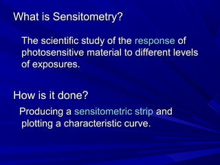
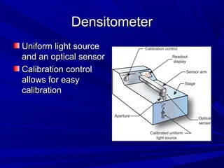
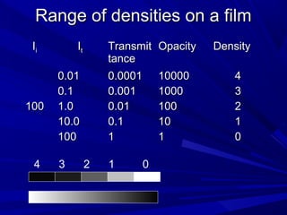
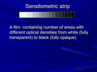
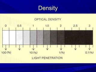
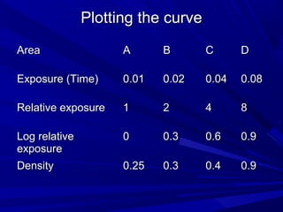
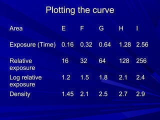
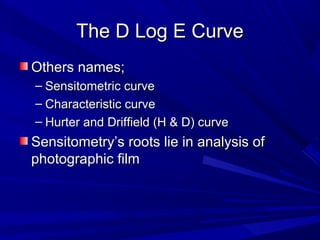
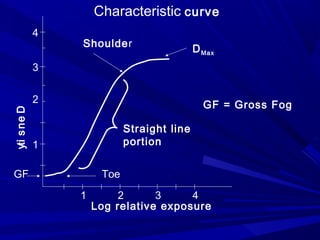
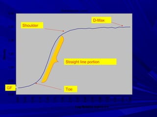
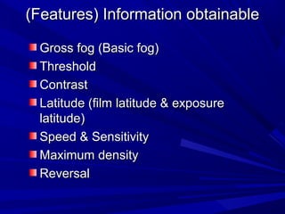
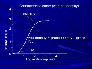
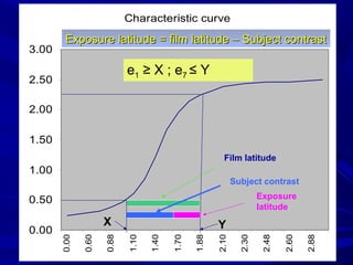
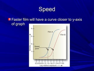
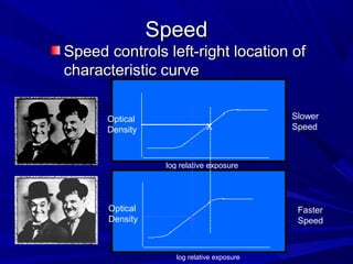
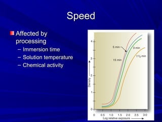
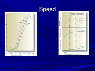
Sensitometry

Quantitive evaluation of how a film
emulsion is responds to radiation
and processing.
‫التقييم الكمى لستجابة الفلم للشعة و‬
‫التحميض‬
Objectives
The student should be able to:
Describe the importance of the study
Define the relevant terms
Describe the methods of producing a
sensitometric strip
Plot the characteristic curve
Describe the Features of the characteristic
curve
Describe the importance & practical
applications
Why is the study important?
To produce images with optimum contrast
that reveal high details of the object
examined.
Optimum contrast?
Low contrast (long scale contrast)
High contrast (Short scale contrast)
Introduction
Photosensitive materials (x-ray films) are
used to record the invisible x-ray image
It is required to reproduce all the
characteristics of the invisible image in
visible form.
The films ability to do so depends on its
sensitometric properties.
It is advantages to have a sound
knowledge of sensitometric properties of
x-ray films.
vi
In

le
ib
s

X-ray tube

Plot of incident x-ray
beam intensity

of
on ge
ti a
a
rm y im
Fo -ra
x

Object
Invisible x-ray
image

Plot of transmitted x-ray
beam intensity
Invisible x-ray image
kV mA Sec FFD
E
Supporting tissue (m)

B
B1

EM

B2

E B1

E B2

T2

T1

ET1

EM

T3

Air

Invisible
X-ray
image

ET2
ET3

EA
What is Sensitometry?
The scientific study of the response of
photosensitive material to different levels
of exposures.

How is it done?
Producing a sensitometric strip and
plotting a characteristic curve.
What is Response of exposure &
How is it manifested?



The response is the change that takes
place, after exposure to electromagnetic
radiation (light or x-rays), in the
photosensitive emulsion on the film

 The response of the film to exposures is
manifested as a degree of blackening
produced after chemical processing
How is degree of blackening
quantified/measured?
1. Transparency (transmission): when

photographic image is held up for light
for inspection it will be observed that it
made up of many varied area of different
brightness.
Intensity of transmitted light
Transparency = ---------------------------------Intensity of incident light
2. Opacity

reciprocal of transparency is known as
opacity.
Intensity of incident light
Opacity = ---------------------------------Intensity of transmitted light
3.

Optical Density (OD)
is expressed as a number that is actually a logarithm,
using the common base 10.
Photographic density is defined by

D

=

(Log of opacity) = log 10 Io / I

D = density. IO light incident on a film. I light transmitted
by the film
How is degree of blackening
quantified/measured?



In Radiography the degree of film
blackening is quantitatively indicated by
the term ‘Optical Density’.



The optical density describes how
much a certain area of the film is opaque
to light incident upon it .
Optical Density
The optical density is expressed
quantitatively as,
Optical Density = Log10 Opacity
It is measured by using the ‘Densitometer’
(The densitometer works on the following
principle)
Consider the light transmitted through an
area of a film

Incident light
intensity (Ii )

Transmitted light
intensity (It )

Transmittance (Transmission ratio)= It / Ii
Opacity = 1 / Transmittance = Ii / It
Density = Log10 Opacity = Log10 I i / It
Densitometer
Uniform light source
and an optical sensor
Calibration control
allows for easy
calibration
Range of densities on a film
Ii

100

4

It

Transmit Opacity
tance

0.01
0.1
1.0
10.0
100
3

0.0001
0.001
0.01
0.1
1
2

1

0

10000
1000
100
10
1

Density
4
3
2
1
0
Sensitometric strip

A film containing number of areas with
different optical densities from white (fully
transparent) to black (fully opaque)
How to produce a sensitometric
strip and the characteristic curve?
1.Expose a film to different amounts of
known exposures starting from a minimum
and increasing at a known rate (ratio /
wedge factor) up to a maximum.
2. Process the film
3. Measure the densities
4. Tabulate the result & Study the response
by plotting a curve (density Vs Log relative
exposure
Methods of exposing
Time scale method
(using x-ray exposure)
Intensity scale method
i. Using x-ray exposure
ii. Using light exposure
Time scale method
The film is exposed to different quantities of
exposures using constant intensity and
variable duration.
(Quantity = Intensity x Time)
Equipment required
X-ray machine
Cassette with film inside
Lead sheets
Processor
Densitometer
Graph paper
Procedure (time scale method)
X-ray tube

Constants
kV, mA, FFD
Variable
Time
Loaded
cassette
Areas to
be
exposed

Loaded cassette

Lead sheets
Exposure selection
Minimum exposure
Low enough not to produce a measurable
density
Maximum exposure
High enough to produce a density around 3.0
Increment
Wedge factor (Ratio between two exposures)
of 2 is adequate. (2½ can be used to get more
levels)
Alternatively the time steps available in the
machine may be used to get more points on
the graph
Intensity scale method 1
Making a single exposure
using
a calibrated step
wedge
X-ray machine
a loaded cassette
(The intensity of x-rays
passing through the
steps are different &
the duration of
exposure is the same)

-ray
X

ure
s
xpo
e
Intensity scale method 2
The film is exposed to a series of different
intensities of light for the same duration
using an instrument called the
“Sensitometer”.
The wedge factor is usually 2½
The colour of light should match the
spectral sensitivity of the film
Sensitometer
Uses a controlled light
source
– Produces same
amount of light each
time it is triggered
Spectral Sensitivity
1

e vi t a e R
l
es n o ps er

This is the term
used to describe
the response of
the film to the
range of
wavelengths
(spectrum of
colours) of light

Monochromatic
film
Orthochro
matic film

0.5

300

400

500 600 700
Wavelength
(nm)
OD examples
T

OD

Comment

1.0000

0

(Perfectly clear (does not exist

0.7760

0.11 (Unexposed film (base + fog

0.1000

1

Medium gray

0.0100

2

Dark

0.0010

3

Very dark; requires hot lamp

0.00025 3.6

Maximum OD used in medical
radiography
Film obtained
using time
scale method
Density
Plotting the curve
Area

A

B

C

D

Exposure (Time)

0.01

0.02

0.04

0.08

Relative exposure

1

2

4

8

Log relative
exposure
Density

0

0.3

0.6

0.9

0.25

0.3

0.4

0.9
Plotting the curve
Area

E

F

G

H

I

Exposure (Time) 0.16

0.32

0.64

1.28 2.56

Relative
exposure

16

32

64

128

256

Log relative
exposure

1.2

1.5

1.8

2.1

2.4

Density

1.45

2.1

2.5

2.7

2.9
The D Log E Curve
Others names;
– Sensitometric curve
– Characteristic curve
– Hurter and Driffield (H & D) curve

Sensitometry’s roots lie in analysis of
photographic film

Copyright © 2006 by Thomson Delmar
Learning. ALL RIGHTS RESERVED.
Characteristic curve
4

Shoulder

D Max

yti s n e D

3
2

GF = Gross Fog
Straight line
portion

1

GF

Toe
1

2
3
4
Log relative exposure
Characteristic curve

3.00

D-Max
Shoulder

2.50

1.50

Straight line portion
1.00

0.50

GF

Toe

Log Relative exposure

3.48

3.35

3.24

3.10

2.88

2.60

2.48

2.30

2.10

1.88

1.70

1.40

1.10

0.88

0.60

0.00
0.00

Density

2.00
(Features) Information obtainable
Gross fog (Basic fog)
Threshold
Contrast
Latitude (film latitude & exposure
latitude)
Speed & Sensitivity
Maximum density
Reversal
Gross fog (Basic fog) & net density
This is the density of the horizontal part of the
curve at the minimum exposure level
Gross fog = Base Density + Fog
Base Density :- Density produced by the base
material
Fog :- Density produced by the development of
silver halide crystals which have not
received an intentional exposure
Net density = Gross density – Gross fog
4

Characteristic curve (with net density)
Shoulder

yti s n e Dt e N

3
2
Net density = gross density – gross
fog

1

Toe
0

1

2
3
4
Log relative exposure
Threshold
The region where the film emulsion begins to
respond to the exposure

Contrast
The rate of change of density for a given change of
log relative exposure
Contrast = ΔD / ΔE
It is given by the slope (gradient) of the straight line
portion of the curve. If it is a true straight line then
the contrast is called Gamma.
Since, in practice, the curve is not an exact straight
line, the average gradient is taken as the contrast.
Characteristic curve
3.00
2.50
2.00
Contrast = ΔD/ ΔE

1.50
ΔD

1.00
0.50

2.88

2.60

2.48

2.30

2.10

1.88

1.70

1.40

1.10

0.88

0.60

0.00

0.00

ΔE
Average gradient

yi s ne D
t

4
3

B

DY
2

1
DX

A

Average gradient = BC/AC
DY - DX
= ----------log E Y – log E X

C

How to select points A and
B ?

Log EX 1 Log EY 2

3
4
Log relative exposure
Point A ? Point B ?
A : DX = 0.25 above Basic fog
B : DY = 2.0 above Basic fog
 The densities from 0.25 to 2.0 is called

the Useful Density range.
 Useful density range is the density range
in which the differences can be identified
by the human eye.
 The densities which represents different
structures on a radiograph should lie
within this range of densities.
Contrast
Contrast controls slope of
characteristic curve
Optical
Density

Lower
Contrast

log relative exposure

Higher
Contrast

Optical
Density

log relative exposure
 Useful

density range is the range of
densities within which the human
eye can recognize the small
differences
That is the range of net densities
from
0.25 to 2.0
Latitude
Latitude is an expression of the tolerance of a
system to extreme conditions of exposure.
It refers to the ability of a film or film-screen
system to record successfully a wide range of
exposure .
(considered in two parts)
Film latitude & Exposure latitude

Film Latitude
The difference between the upper and
lower limits of log relative exposure which
produce densities within the useful range
Significance of film latitude
The range of x-ray intensities transmitted
through the body part should lie within the
film latitude, if they are to be viewed as
useful densities on the radiograph.
Any x-ray intensity that falls out side the
film latitude will not reveal any information
& a useful piece of information might be
lost
Film latitude & Average gradient

yi s ne D
t

4
3

DY
2

1
DX

B

A

C

Log EX 1 Log EY 2

Film latitude

When Dx = 0.25+BF & Dy = 2.0
+BF
DY - DX
Average gradient = ----------becomes
log E Y – log
EX
1.75
= -----------------3
4 Film latitude
Log relative exposure
Exposure latitude
This refers to the freedom of the
radiographer to select slightly different
exposures (to make room for errors) for a
particular examination so that the resulted
densities remains within the useful density
range.
Exposure latitude = film latitude – subject
contrast (log relative exposure range
transmitted from a particular body part)
Subject contrast
kV mA Sec FFD
E

B
B

E1

Air

E2

E3

E4

E5

E6

E7
Transmitted
intensities

E1

Relative
Intensity
Log relative
intensity

E2

E3

E4

E5

E6

RE1 RE2

RE3

RE4

RE5

RE6 RE7

e1

e3

e4

e5

e6

e2

e7

e1
Subject contrast

E7
e7
Image contrast

e1

D1 D2

e7

D3

D4 D5

D6

D7
Characteristic curve
3.00

Exposure latitude = film latitude – Subject contrast

e1 ≥ X ; e7 ≤ Y

2.50
2.00
1.50

Film latitude

1.00
Subject contrast
Exposure
latitude

0.50

2.88

2.60

2.48

2.30

2.10

1.88

1.70

1.40

Y
1.10

0.88

0.60

0.00

0.00

X
Speed & Sensitivity
 Sensitivity refers to the exposure required
by a film or film-screen system to produce
a net density of 1.
 Sensitivity is expressed in miliroentgens
(mR)
 A high sensitive (have low mR value for
sensitivity) or high speed system requires
less exposure than that of a low sensitive
or low speed system.
Speed
Numerically the Speed
is proportional to the
reciprocal of the
sensitivity (mR) and
is expressed as
128
Speed = -------------Sensitivity (mR)

Sensitivity
(mR)

1200

0.1

800

0.16

400

0.32

200

0.64

100

1.28

50

2.56

25

5.0

12

10.0
yi s ne D
t

4

Comparison of Speeds of two films (filmscreen systems)
A

3
2

B
Speed A > Speed B

1+BF

Speed A α 1/ E SA
Speed B α 1/ E SB

1

Speed A
-------------

BF
1
2
3
Log ESA
Log ESB

=

E SB
------

Speed B
E SA
4
Log relative exposure
Speed
Faster film will have a curve closer to y-axis
of graph
Speed
Speed controls left-right location of
characteristic curve
Optical
Density

X

Slower
Speed

log relative exposure

Optical
Density

X

log relative exposure

Faster
Speed
Speed
Affected by
processing
– Immersion time
– Solution temperature
– Chemical activity
Speed
Maximum Density (DMax)
The density produced when all the silver
bromide crystals in the emulsion is
exposed and developed

Reversal
This is the region where the density
reduces with the increasing exposure
greater than that produce DMax
yi s ne D
t

4

D Max & Reversal
DMax

3
Reversal

2

1
BF
1

2

3

4
Log relative exposure
Reversal or Solarization
Once a film has been
exposed to Dmax, it will
begin to lose density
after further exposure
Duplication film has
been solarized
Uses of the characteristic curve
Information
Gross fog (Basic fog)
Threshold
Contrast
Latitude (film latitude &
exposure latitude)
Speed & Sensitivity
Maximum density
Reversal

Uses
Selection of films
Assessing processor
performance (Quality
control)
Selection of exposure
factors
Comparison of filmscreen systems
Duplication of
radiographs
Summary
Definitions of terms
Methods of producing a sensitometric
strip
Plotting the Characteristic curve
Features of the characteristic curve
The practical applications
Thank You

Sensitometry3

  • 1.
    Sensitometry Quantitive evaluation ofhow a film emulsion is responds to radiation and processing. ‫التقييم الكمى لستجابة الفلم للشعة و‬ ‫التحميض‬
  • 2.
    Objectives The student shouldbe able to: Describe the importance of the study Define the relevant terms Describe the methods of producing a sensitometric strip Plot the characteristic curve Describe the Features of the characteristic curve Describe the importance & practical applications
  • 3.
    Why is thestudy important? To produce images with optimum contrast that reveal high details of the object examined. Optimum contrast? Low contrast (long scale contrast) High contrast (Short scale contrast)
  • 4.
    Introduction Photosensitive materials (x-rayfilms) are used to record the invisible x-ray image It is required to reproduce all the characteristics of the invisible image in visible form. The films ability to do so depends on its sensitometric properties. It is advantages to have a sound knowledge of sensitometric properties of x-ray films.
  • 5.
    vi In le ib s X-ray tube Plot ofincident x-ray beam intensity of on ge ti a a rm y im Fo -ra x Object Invisible x-ray image Plot of transmitted x-ray beam intensity
  • 6.
    Invisible x-ray image kVmA Sec FFD E Supporting tissue (m) B B1 EM B2 E B1 E B2 T2 T1 ET1 EM T3 Air Invisible X-ray image ET2 ET3 EA
  • 7.
    What is Sensitometry? Thescientific study of the response of photosensitive material to different levels of exposures. How is it done? Producing a sensitometric strip and plotting a characteristic curve.
  • 8.
    What is Responseof exposure & How is it manifested?  The response is the change that takes place, after exposure to electromagnetic radiation (light or x-rays), in the photosensitive emulsion on the film  The response of the film to exposures is manifested as a degree of blackening produced after chemical processing
  • 9.
    How is degreeof blackening quantified/measured? 1. Transparency (transmission): when photographic image is held up for light for inspection it will be observed that it made up of many varied area of different brightness. Intensity of transmitted light Transparency = ---------------------------------Intensity of incident light
  • 10.
    2. Opacity reciprocal oftransparency is known as opacity. Intensity of incident light Opacity = ---------------------------------Intensity of transmitted light
  • 11.
    3. Optical Density (OD) isexpressed as a number that is actually a logarithm, using the common base 10. Photographic density is defined by D = (Log of opacity) = log 10 Io / I D = density. IO light incident on a film. I light transmitted by the film
  • 12.
    How is degreeof blackening quantified/measured?  In Radiography the degree of film blackening is quantitatively indicated by the term ‘Optical Density’.  The optical density describes how much a certain area of the film is opaque to light incident upon it .
  • 13.
    Optical Density The opticaldensity is expressed quantitatively as, Optical Density = Log10 Opacity It is measured by using the ‘Densitometer’ (The densitometer works on the following principle)
  • 14.
    Consider the lighttransmitted through an area of a film Incident light intensity (Ii ) Transmitted light intensity (It ) Transmittance (Transmission ratio)= It / Ii Opacity = 1 / Transmittance = Ii / It Density = Log10 Opacity = Log10 I i / It
  • 15.
    Densitometer Uniform light source andan optical sensor Calibration control allows for easy calibration
  • 16.
    Range of densitieson a film Ii 100 4 It Transmit Opacity tance 0.01 0.1 1.0 10.0 100 3 0.0001 0.001 0.01 0.1 1 2 1 0 10000 1000 100 10 1 Density 4 3 2 1 0
  • 17.
    Sensitometric strip A filmcontaining number of areas with different optical densities from white (fully transparent) to black (fully opaque)
  • 18.
    How to producea sensitometric strip and the characteristic curve? 1.Expose a film to different amounts of known exposures starting from a minimum and increasing at a known rate (ratio / wedge factor) up to a maximum. 2. Process the film 3. Measure the densities 4. Tabulate the result & Study the response by plotting a curve (density Vs Log relative exposure
  • 19.
    Methods of exposing Timescale method (using x-ray exposure) Intensity scale method i. Using x-ray exposure ii. Using light exposure
  • 20.
    Time scale method Thefilm is exposed to different quantities of exposures using constant intensity and variable duration. (Quantity = Intensity x Time) Equipment required X-ray machine Cassette with film inside Lead sheets Processor Densitometer Graph paper
  • 21.
    Procedure (time scalemethod) X-ray tube Constants kV, mA, FFD Variable Time Loaded cassette Areas to be exposed Loaded cassette Lead sheets
  • 22.
    Exposure selection Minimum exposure Lowenough not to produce a measurable density Maximum exposure High enough to produce a density around 3.0 Increment Wedge factor (Ratio between two exposures) of 2 is adequate. (2½ can be used to get more levels) Alternatively the time steps available in the machine may be used to get more points on the graph
  • 23.
    Intensity scale method1 Making a single exposure using a calibrated step wedge X-ray machine a loaded cassette (The intensity of x-rays passing through the steps are different & the duration of exposure is the same) -ray X ure s xpo e
  • 24.
    Intensity scale method2 The film is exposed to a series of different intensities of light for the same duration using an instrument called the “Sensitometer”. The wedge factor is usually 2½ The colour of light should match the spectral sensitivity of the film
  • 25.
    Sensitometer Uses a controlledlight source – Produces same amount of light each time it is triggered
  • 26.
    Spectral Sensitivity 1 e vit a e R l es n o ps er This is the term used to describe the response of the film to the range of wavelengths (spectrum of colours) of light Monochromatic film Orthochro matic film 0.5 300 400 500 600 700 Wavelength (nm)
  • 27.
    OD examples T OD Comment 1.0000 0 (Perfectly clear(does not exist 0.7760 0.11 (Unexposed film (base + fog 0.1000 1 Medium gray 0.0100 2 Dark 0.0010 3 Very dark; requires hot lamp 0.00025 3.6 Maximum OD used in medical radiography
  • 28.
  • 29.
  • 30.
    Plotting the curve Area A B C D Exposure(Time) 0.01 0.02 0.04 0.08 Relative exposure 1 2 4 8 Log relative exposure Density 0 0.3 0.6 0.9 0.25 0.3 0.4 0.9
  • 31.
    Plotting the curve Area E F G H I Exposure(Time) 0.16 0.32 0.64 1.28 2.56 Relative exposure 16 32 64 128 256 Log relative exposure 1.2 1.5 1.8 2.1 2.4 Density 1.45 2.1 2.5 2.7 2.9
  • 32.
    The D LogE Curve Others names; – Sensitometric curve – Characteristic curve – Hurter and Driffield (H & D) curve Sensitometry’s roots lie in analysis of photographic film Copyright © 2006 by Thomson Delmar Learning. ALL RIGHTS RESERVED.
  • 33.
    Characteristic curve 4 Shoulder D Max ytis n e D 3 2 GF = Gross Fog Straight line portion 1 GF Toe 1 2 3 4 Log relative exposure
  • 34.
    Characteristic curve 3.00 D-Max Shoulder 2.50 1.50 Straight lineportion 1.00 0.50 GF Toe Log Relative exposure 3.48 3.35 3.24 3.10 2.88 2.60 2.48 2.30 2.10 1.88 1.70 1.40 1.10 0.88 0.60 0.00 0.00 Density 2.00
  • 35.
    (Features) Information obtainable Grossfog (Basic fog) Threshold Contrast Latitude (film latitude & exposure latitude) Speed & Sensitivity Maximum density Reversal
  • 36.
    Gross fog (Basicfog) & net density This is the density of the horizontal part of the curve at the minimum exposure level Gross fog = Base Density + Fog Base Density :- Density produced by the base material Fog :- Density produced by the development of silver halide crystals which have not received an intentional exposure Net density = Gross density – Gross fog
  • 37.
    4 Characteristic curve (withnet density) Shoulder yti s n e Dt e N 3 2 Net density = gross density – gross fog 1 Toe 0 1 2 3 4 Log relative exposure
  • 38.
    Threshold The region wherethe film emulsion begins to respond to the exposure Contrast The rate of change of density for a given change of log relative exposure Contrast = ΔD / ΔE It is given by the slope (gradient) of the straight line portion of the curve. If it is a true straight line then the contrast is called Gamma. Since, in practice, the curve is not an exact straight line, the average gradient is taken as the contrast.
  • 39.
    Characteristic curve 3.00 2.50 2.00 Contrast =ΔD/ ΔE 1.50 ΔD 1.00 0.50 2.88 2.60 2.48 2.30 2.10 1.88 1.70 1.40 1.10 0.88 0.60 0.00 0.00 ΔE
  • 40.
    Average gradient yi sne D t 4 3 B DY 2 1 DX A Average gradient = BC/AC DY - DX = ----------log E Y – log E X C How to select points A and B ? Log EX 1 Log EY 2 3 4 Log relative exposure
  • 41.
    Point A ?Point B ? A : DX = 0.25 above Basic fog B : DY = 2.0 above Basic fog  The densities from 0.25 to 2.0 is called the Useful Density range.  Useful density range is the density range in which the differences can be identified by the human eye.  The densities which represents different structures on a radiograph should lie within this range of densities.
  • 42.
    Contrast Contrast controls slopeof characteristic curve Optical Density Lower Contrast log relative exposure Higher Contrast Optical Density log relative exposure
  • 43.
     Useful density rangeis the range of densities within which the human eye can recognize the small differences That is the range of net densities from 0.25 to 2.0
  • 44.
    Latitude Latitude is anexpression of the tolerance of a system to extreme conditions of exposure. It refers to the ability of a film or film-screen system to record successfully a wide range of exposure . (considered in two parts) Film latitude & Exposure latitude Film Latitude The difference between the upper and lower limits of log relative exposure which produce densities within the useful range
  • 45.
    Significance of filmlatitude The range of x-ray intensities transmitted through the body part should lie within the film latitude, if they are to be viewed as useful densities on the radiograph. Any x-ray intensity that falls out side the film latitude will not reveal any information & a useful piece of information might be lost
  • 46.
    Film latitude &Average gradient yi s ne D t 4 3 DY 2 1 DX B A C Log EX 1 Log EY 2 Film latitude When Dx = 0.25+BF & Dy = 2.0 +BF DY - DX Average gradient = ----------becomes log E Y – log EX 1.75 = -----------------3 4 Film latitude Log relative exposure
  • 47.
    Exposure latitude This refersto the freedom of the radiographer to select slightly different exposures (to make room for errors) for a particular examination so that the resulted densities remains within the useful density range. Exposure latitude = film latitude – subject contrast (log relative exposure range transmitted from a particular body part)
  • 48.
    Subject contrast kV mASec FFD E B B E1 Air E2 E3 E4 E5 E6 E7
  • 49.
  • 50.
  • 51.
    Characteristic curve 3.00 Exposure latitude= film latitude – Subject contrast e1 ≥ X ; e7 ≤ Y 2.50 2.00 1.50 Film latitude 1.00 Subject contrast Exposure latitude 0.50 2.88 2.60 2.48 2.30 2.10 1.88 1.70 1.40 Y 1.10 0.88 0.60 0.00 0.00 X
  • 52.
    Speed & Sensitivity Sensitivity refers to the exposure required by a film or film-screen system to produce a net density of 1.  Sensitivity is expressed in miliroentgens (mR)  A high sensitive (have low mR value for sensitivity) or high speed system requires less exposure than that of a low sensitive or low speed system.
  • 53.
    Speed Numerically the Speed isproportional to the reciprocal of the sensitivity (mR) and is expressed as 128 Speed = -------------Sensitivity (mR) Sensitivity (mR) 1200 0.1 800 0.16 400 0.32 200 0.64 100 1.28 50 2.56 25 5.0 12 10.0
  • 54.
    yi s neD t 4 Comparison of Speeds of two films (filmscreen systems) A 3 2 B Speed A > Speed B 1+BF Speed A α 1/ E SA Speed B α 1/ E SB 1 Speed A ------------- BF 1 2 3 Log ESA Log ESB = E SB ------ Speed B E SA 4 Log relative exposure
  • 55.
    Speed Faster film willhave a curve closer to y-axis of graph
  • 56.
    Speed Speed controls left-rightlocation of characteristic curve Optical Density X Slower Speed log relative exposure Optical Density X log relative exposure Faster Speed
  • 57.
    Speed Affected by processing – Immersiontime – Solution temperature – Chemical activity
  • 58.
  • 59.
    Maximum Density (DMax) Thedensity produced when all the silver bromide crystals in the emulsion is exposed and developed Reversal This is the region where the density reduces with the increasing exposure greater than that produce DMax
  • 60.
    yi s neD t 4 D Max & Reversal DMax 3 Reversal 2 1 BF 1 2 3 4 Log relative exposure
  • 61.
    Reversal or Solarization Oncea film has been exposed to Dmax, it will begin to lose density after further exposure Duplication film has been solarized
  • 62.
    Uses of thecharacteristic curve Information Gross fog (Basic fog) Threshold Contrast Latitude (film latitude & exposure latitude) Speed & Sensitivity Maximum density Reversal Uses Selection of films Assessing processor performance (Quality control) Selection of exposure factors Comparison of filmscreen systems Duplication of radiographs
  • 63.
    Summary Definitions of terms Methodsof producing a sensitometric strip Plotting the Characteristic curve Features of the characteristic curve The practical applications
  • 64.