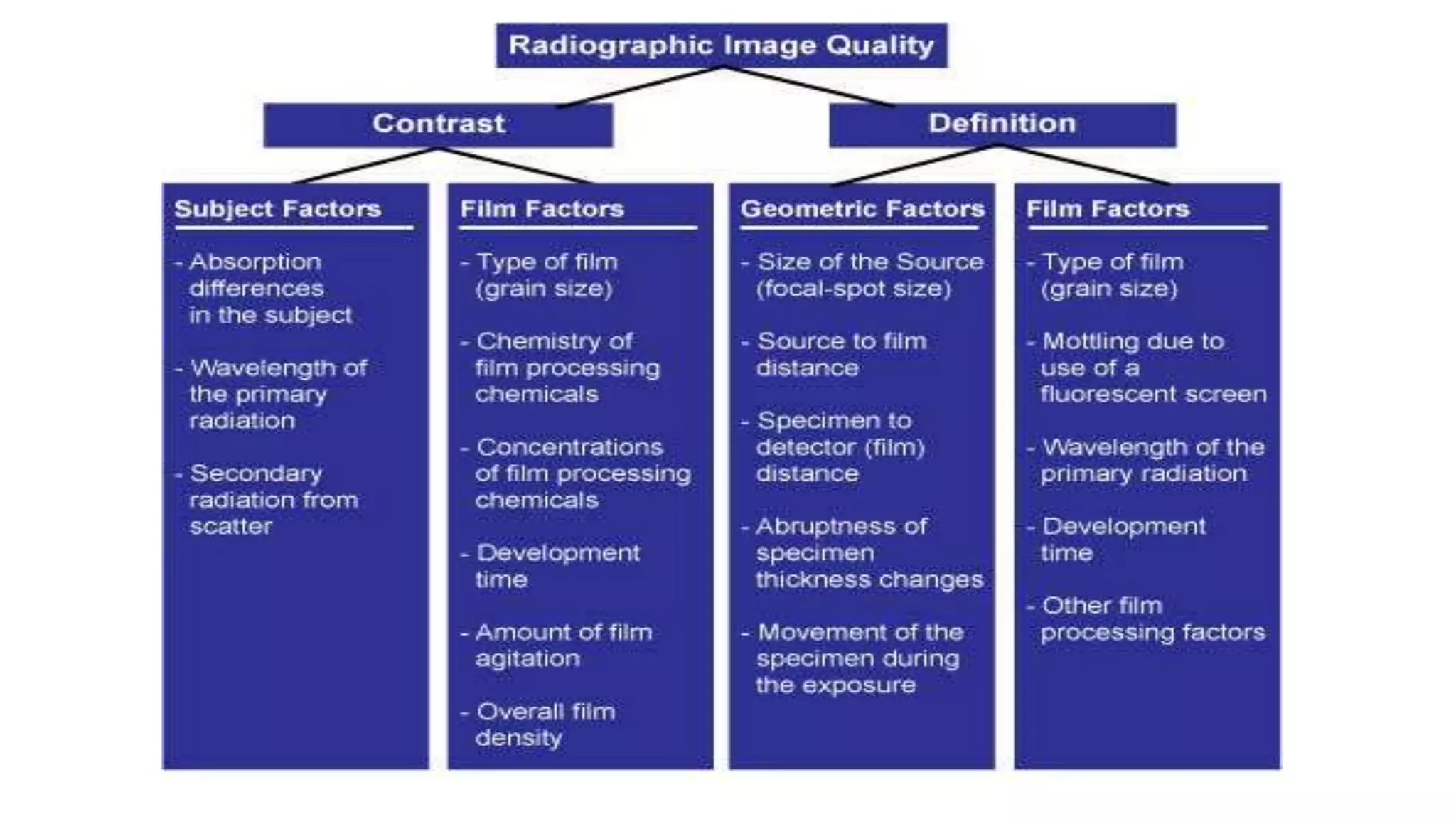
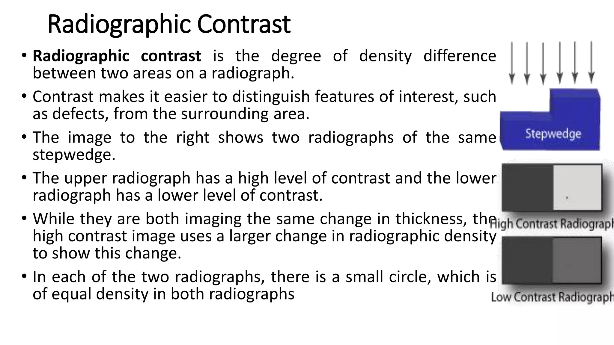
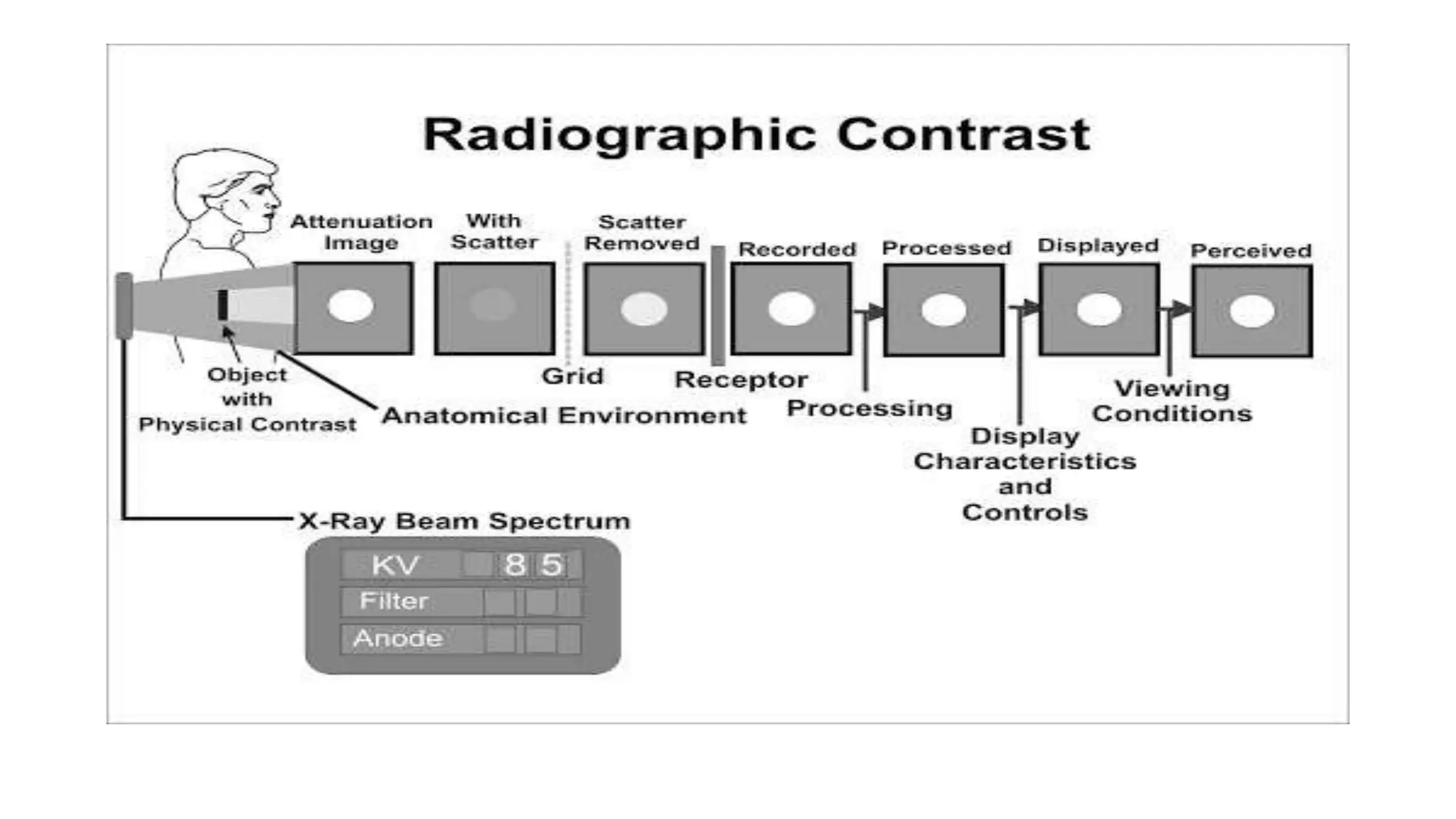
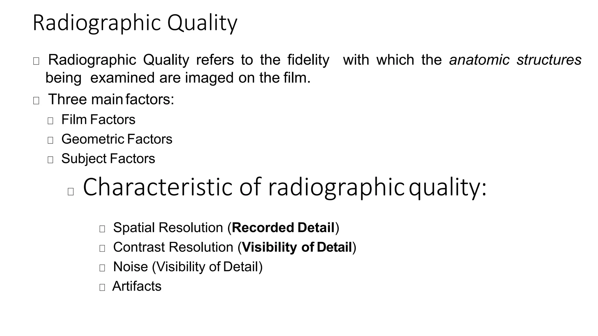
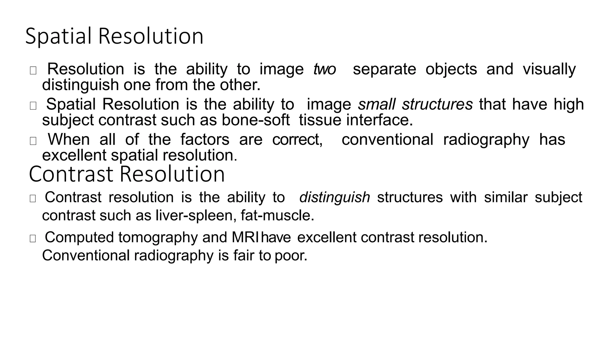
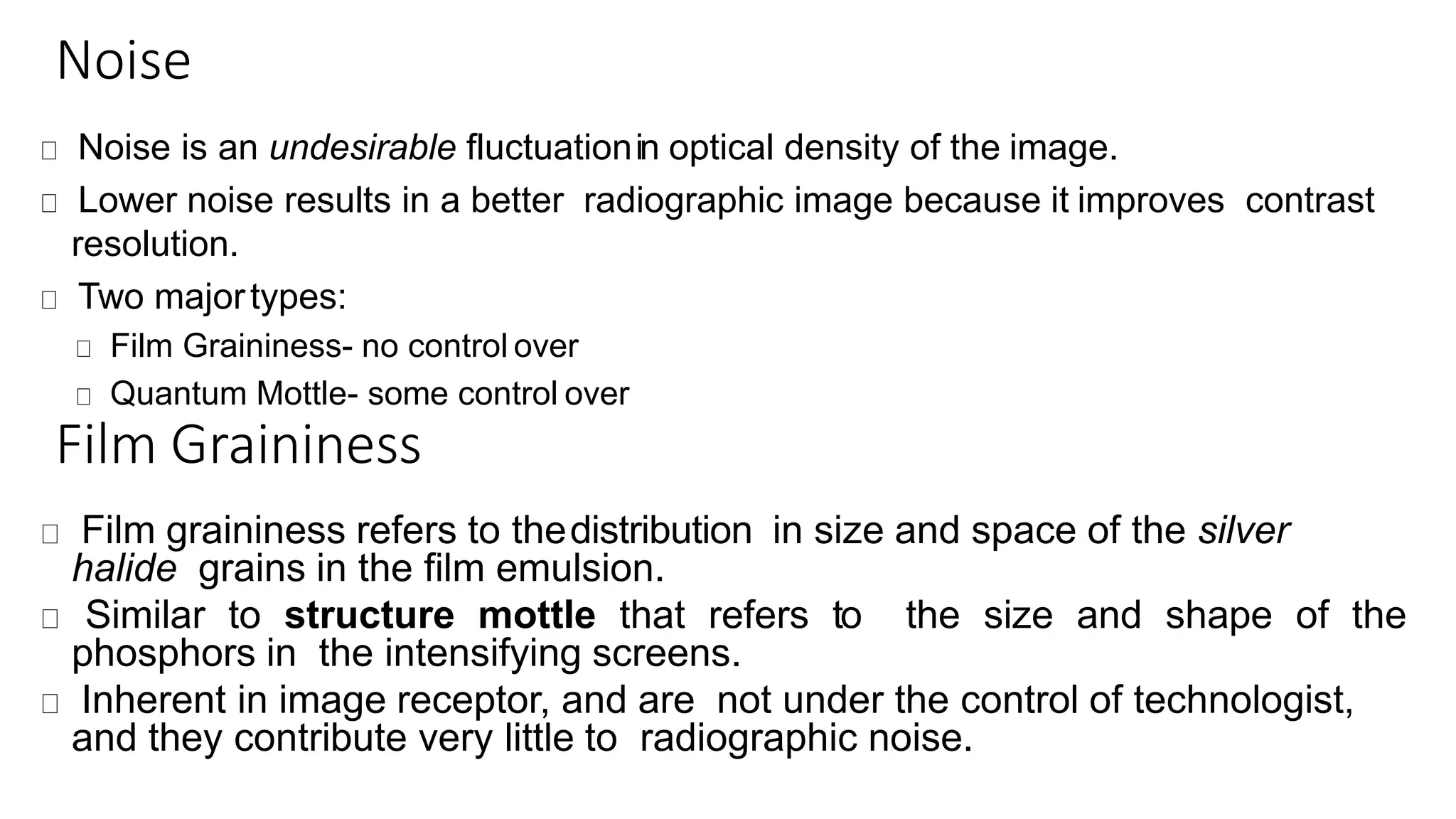
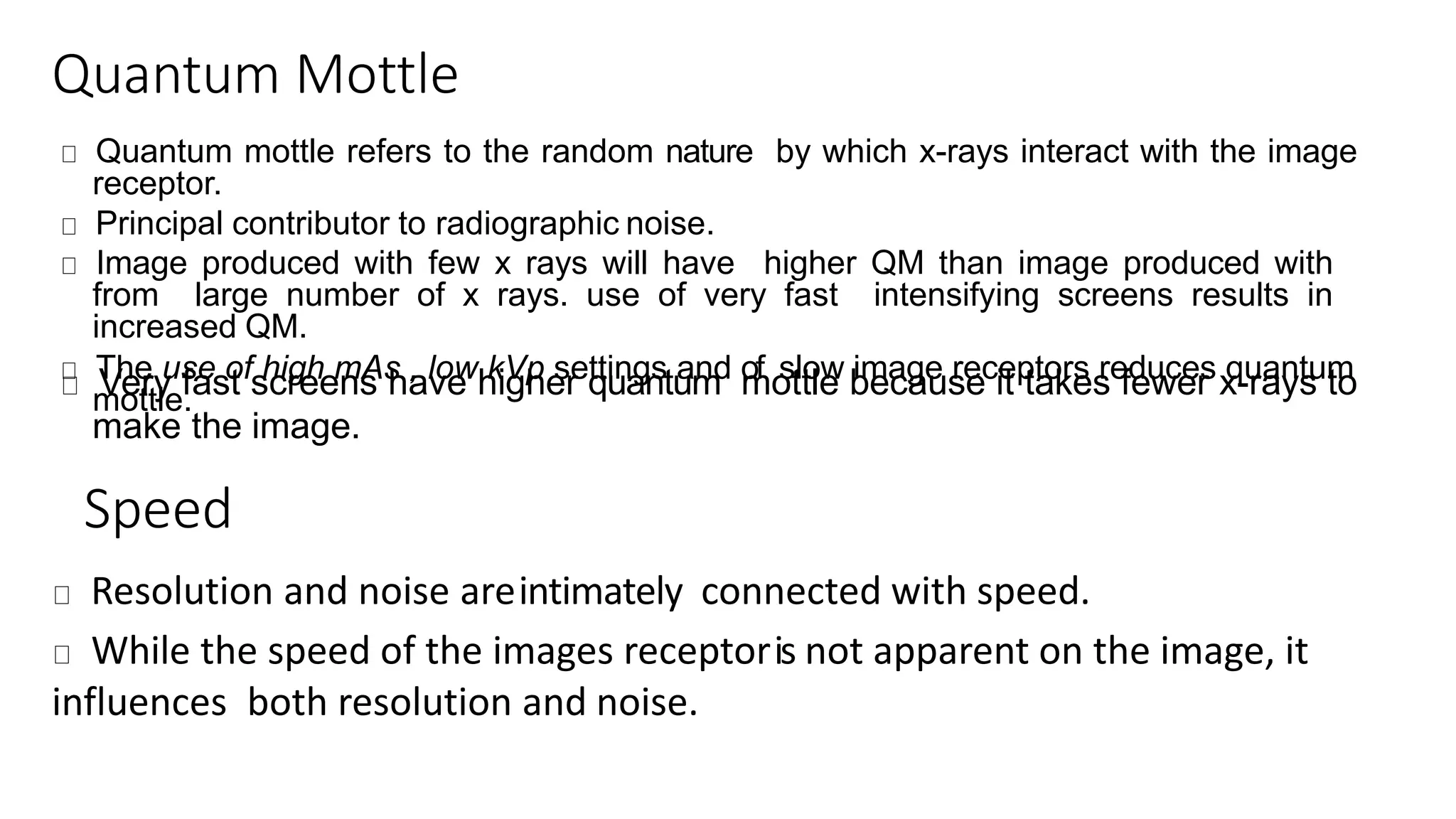
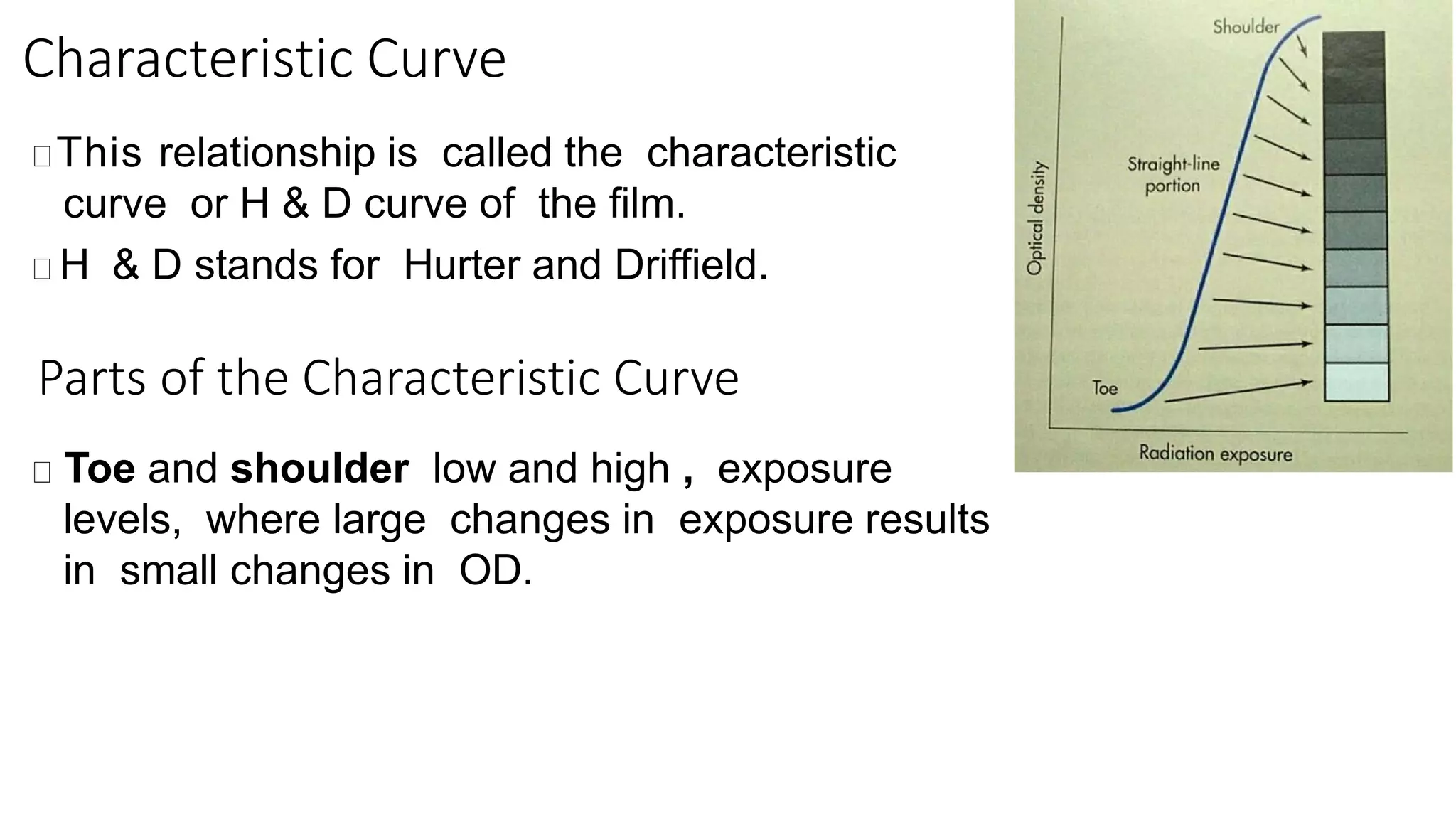
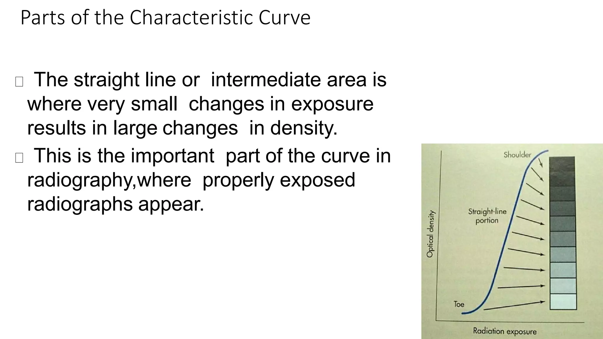
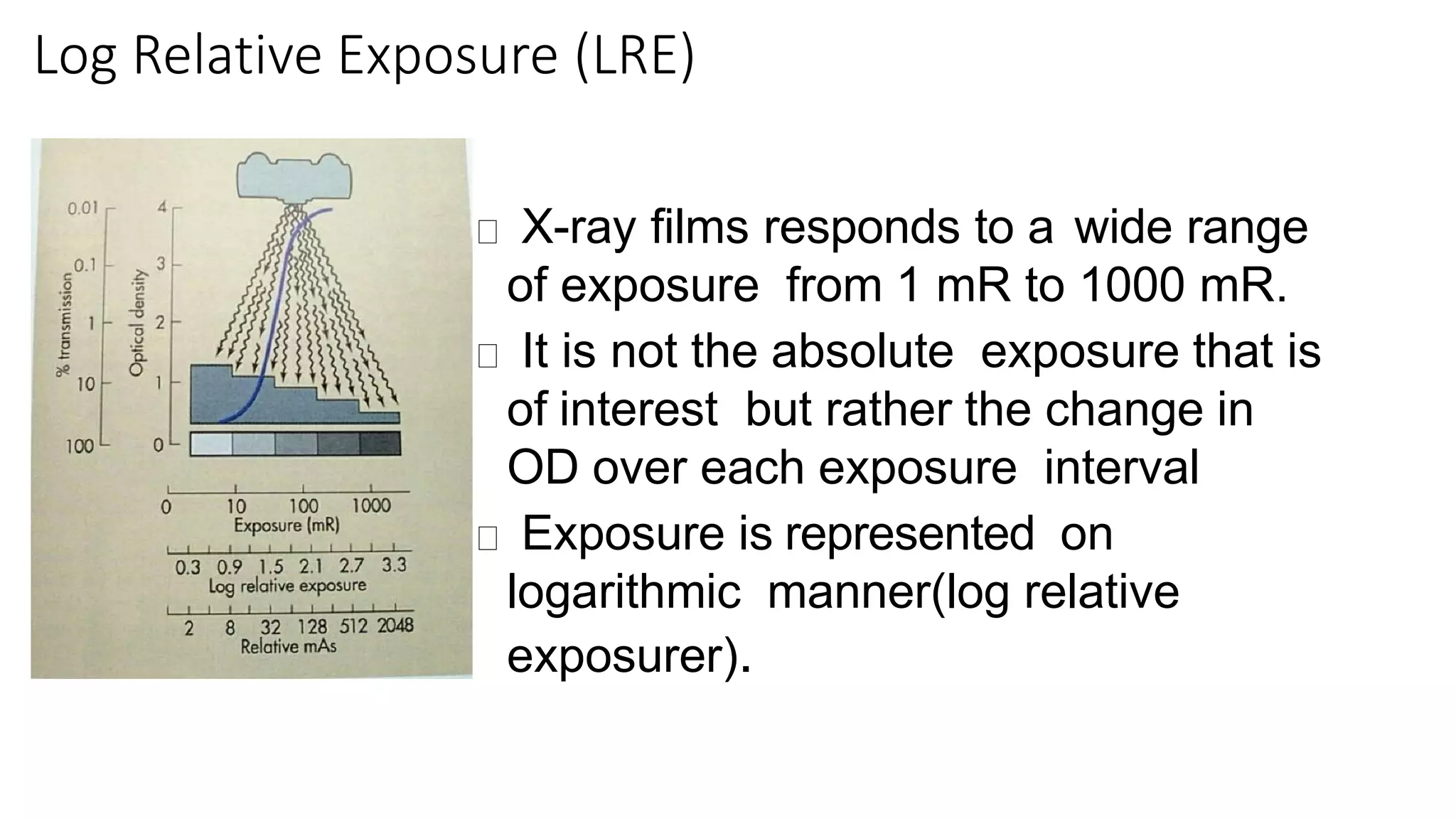
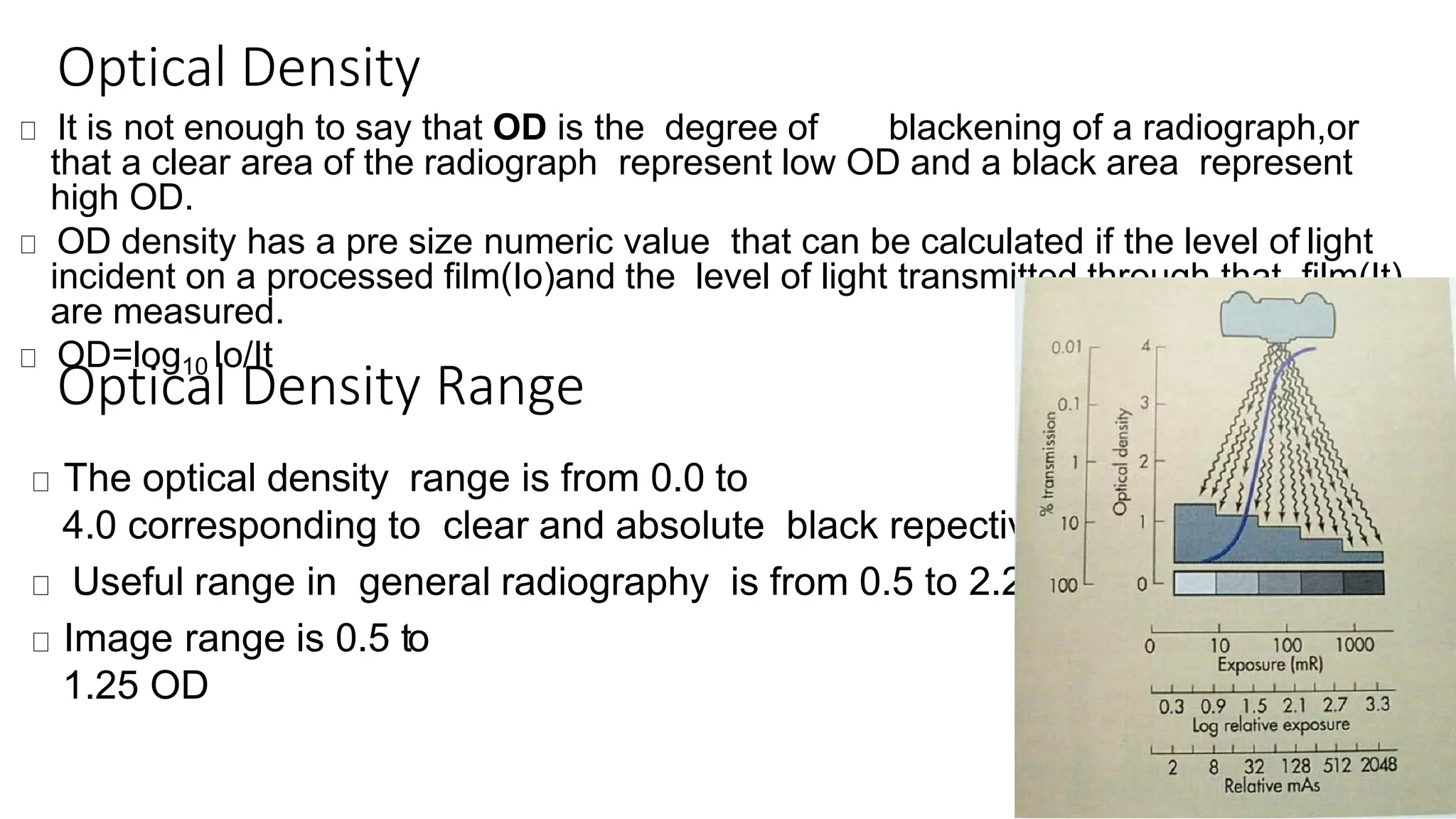
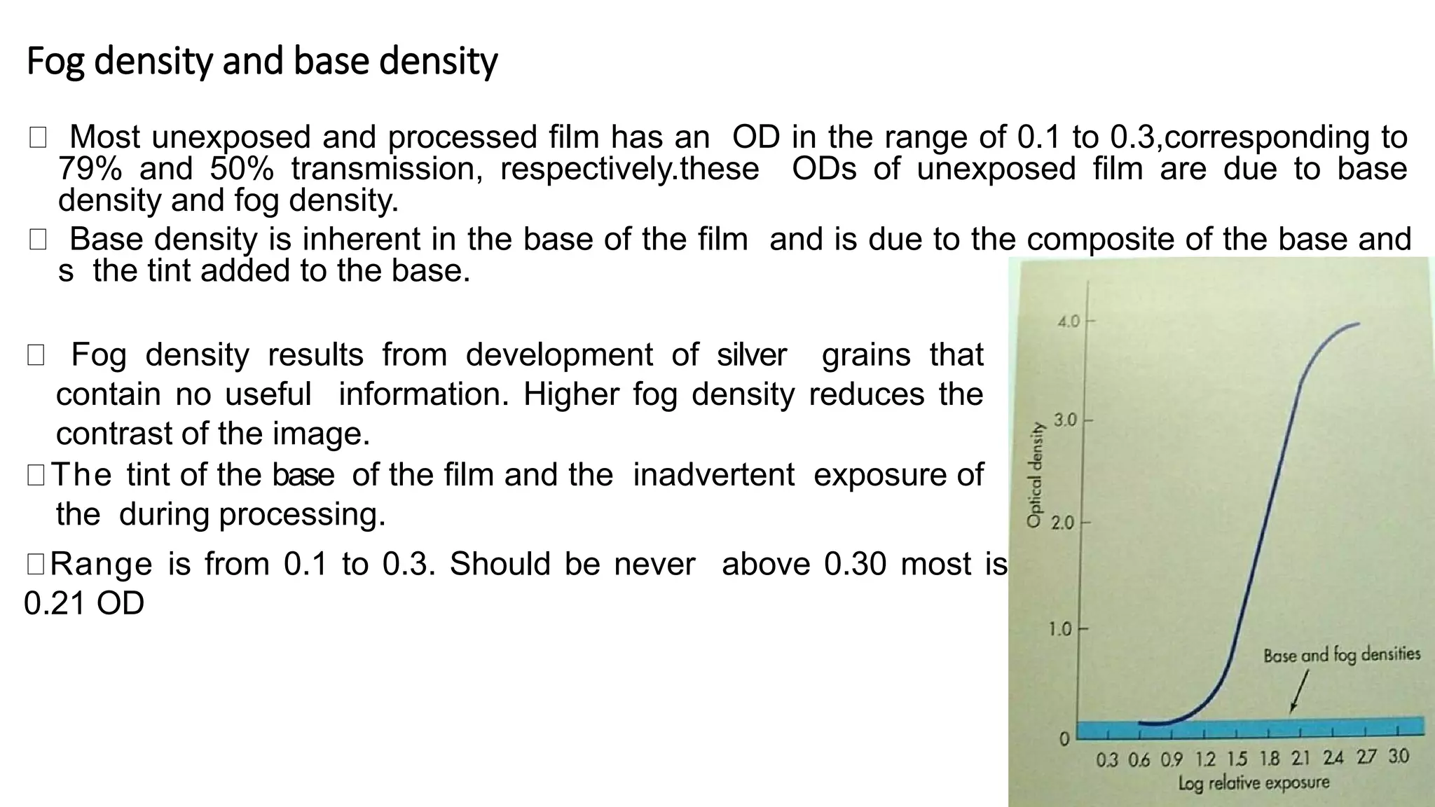
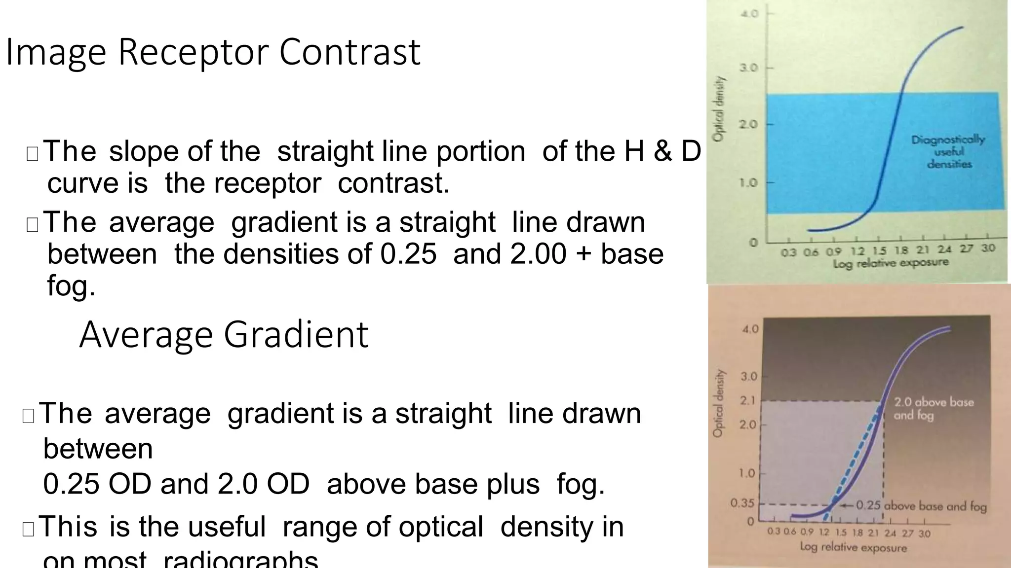
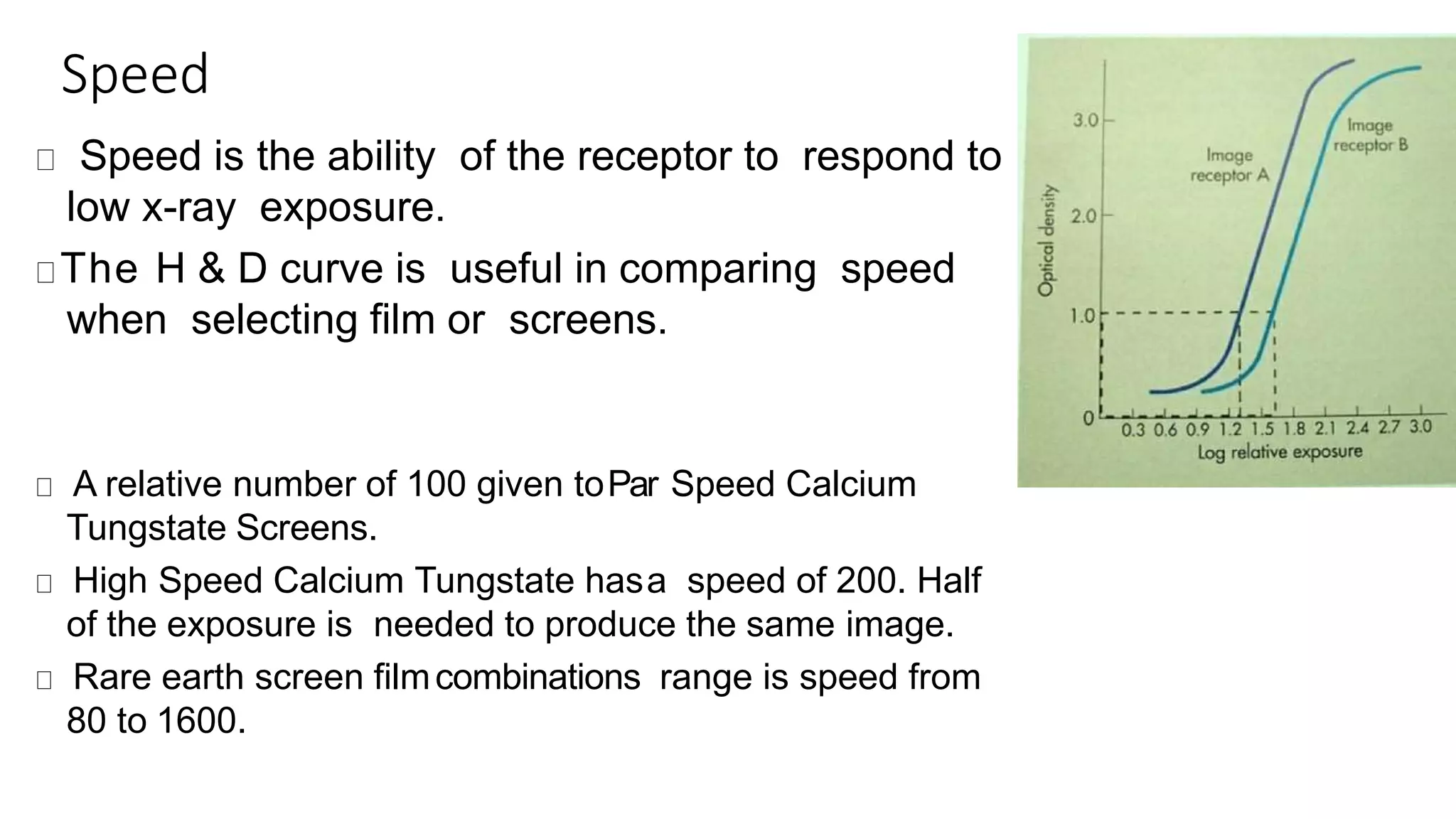
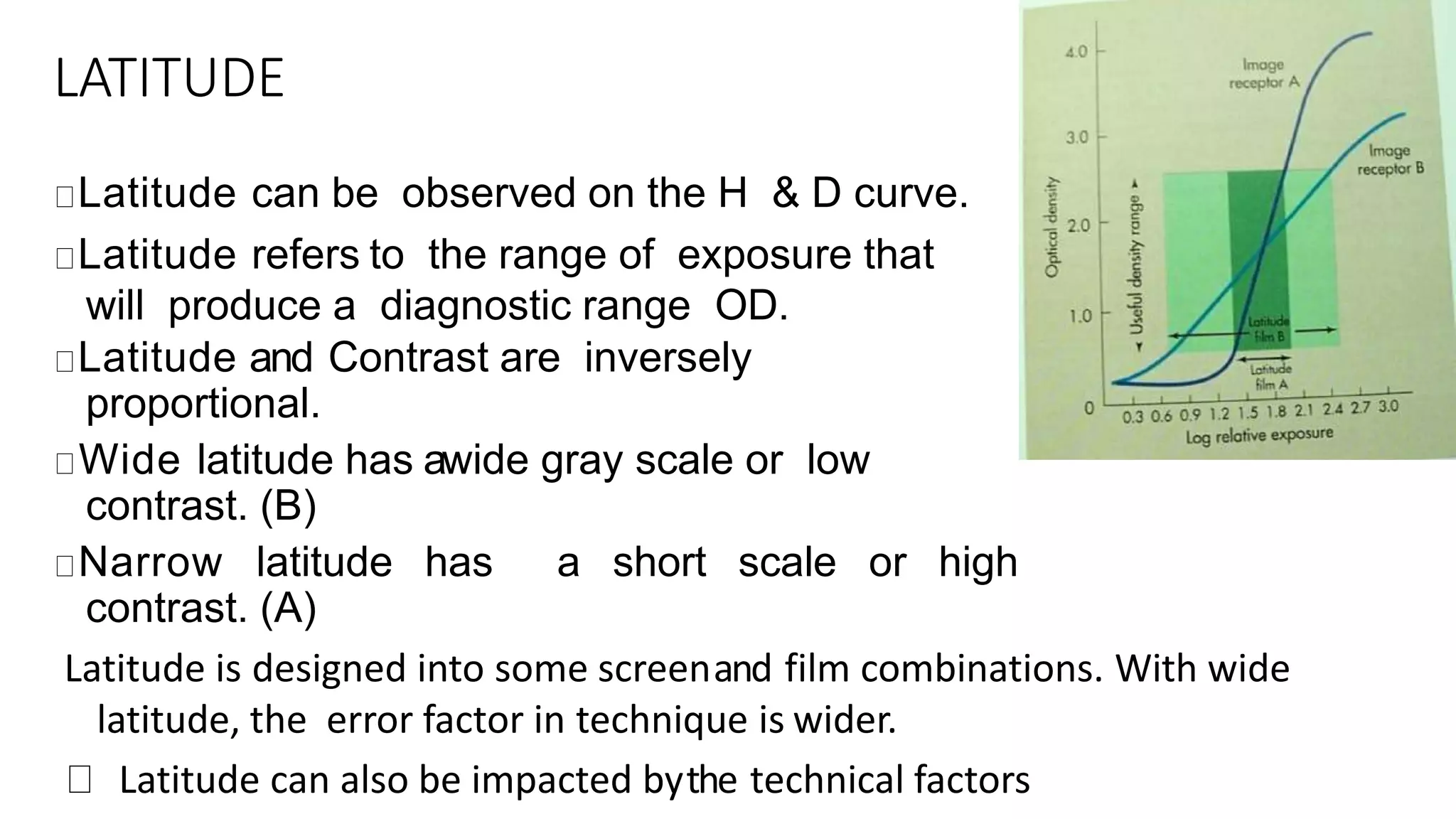
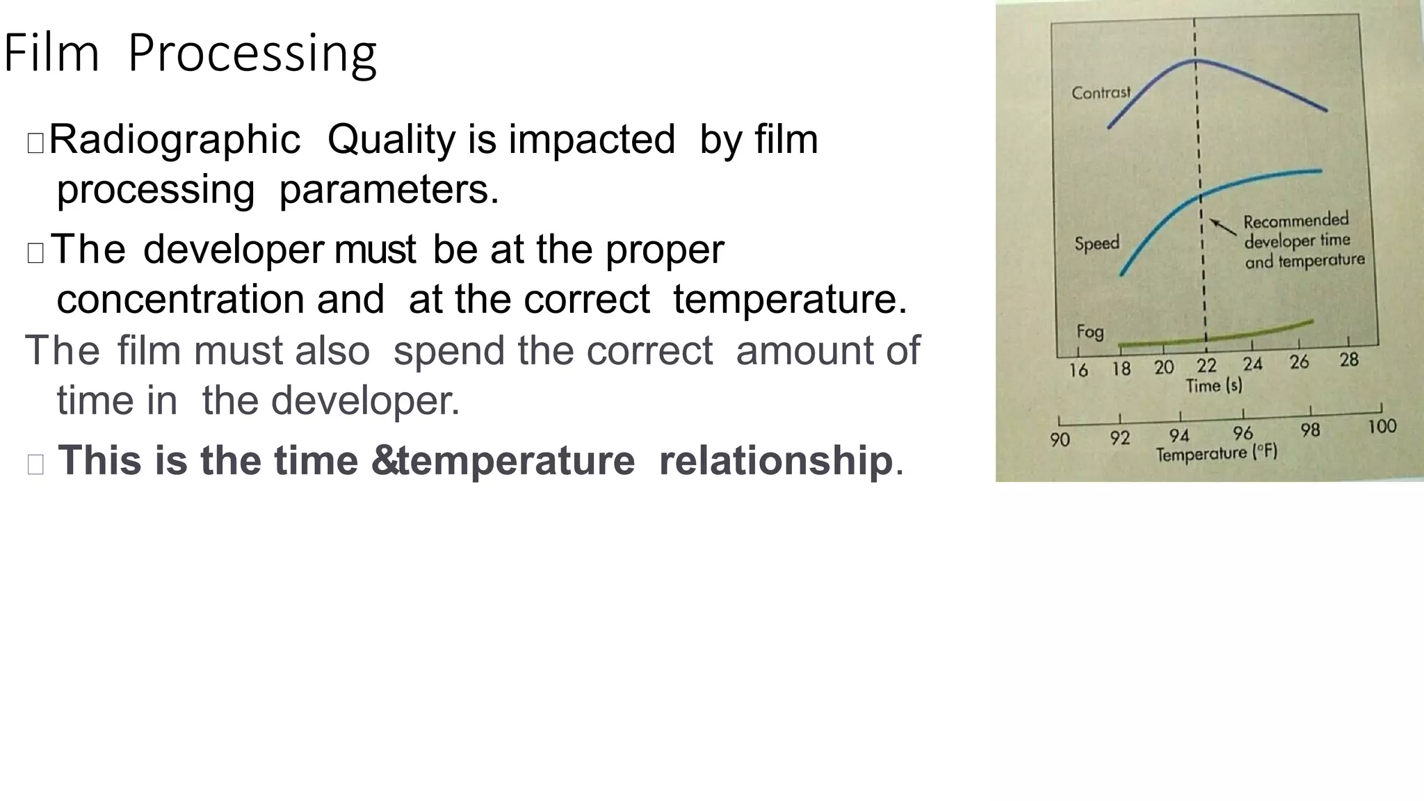
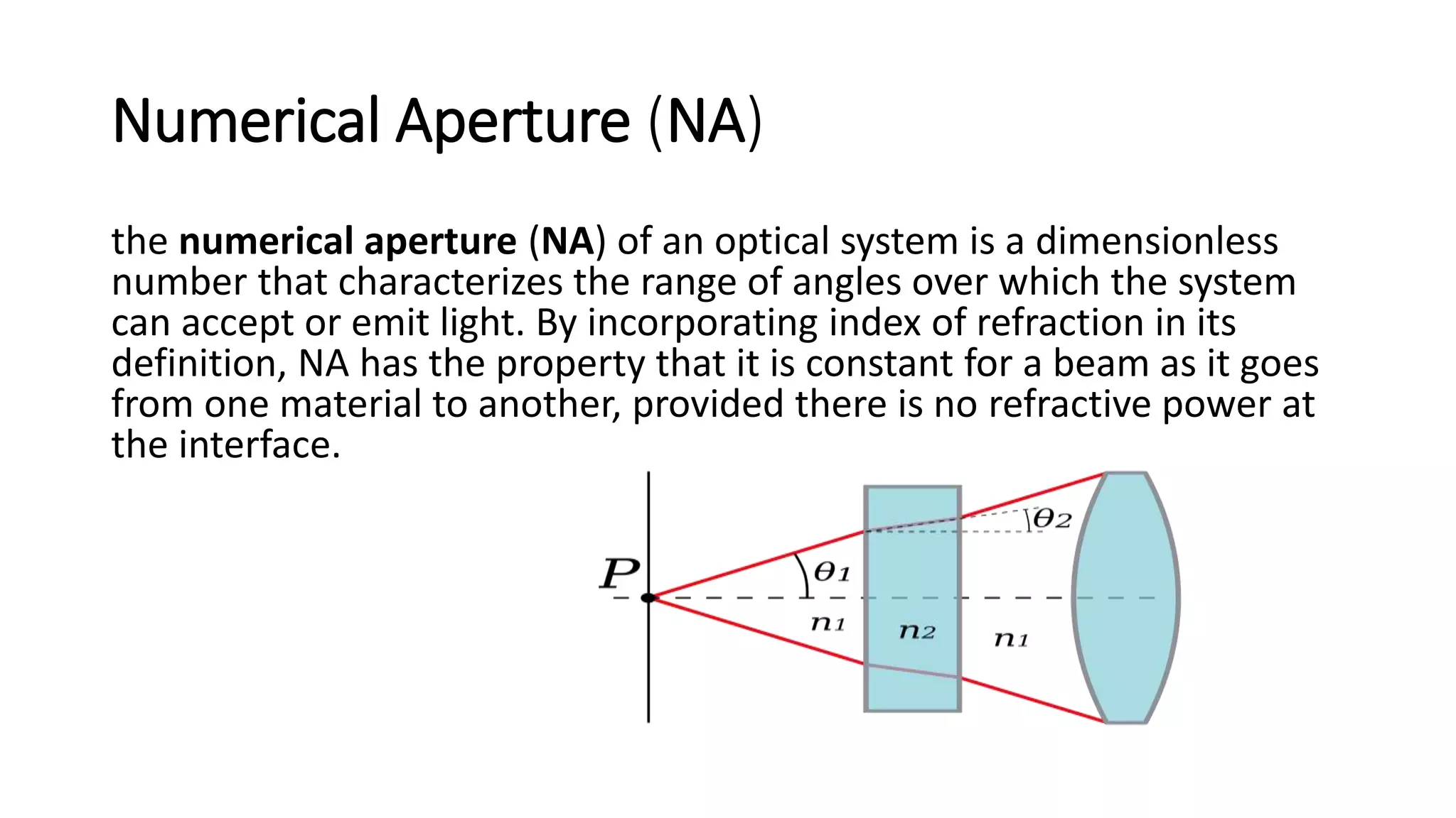
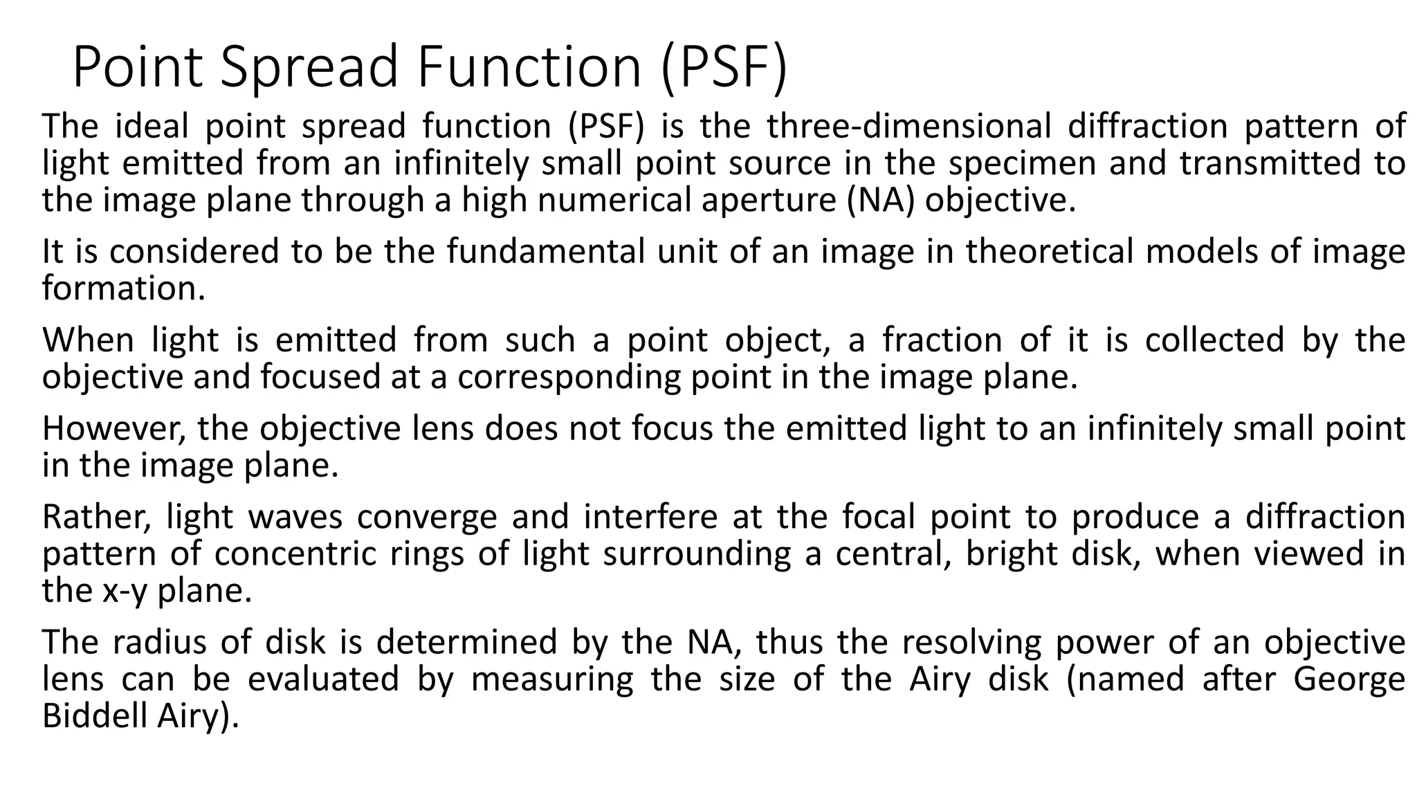
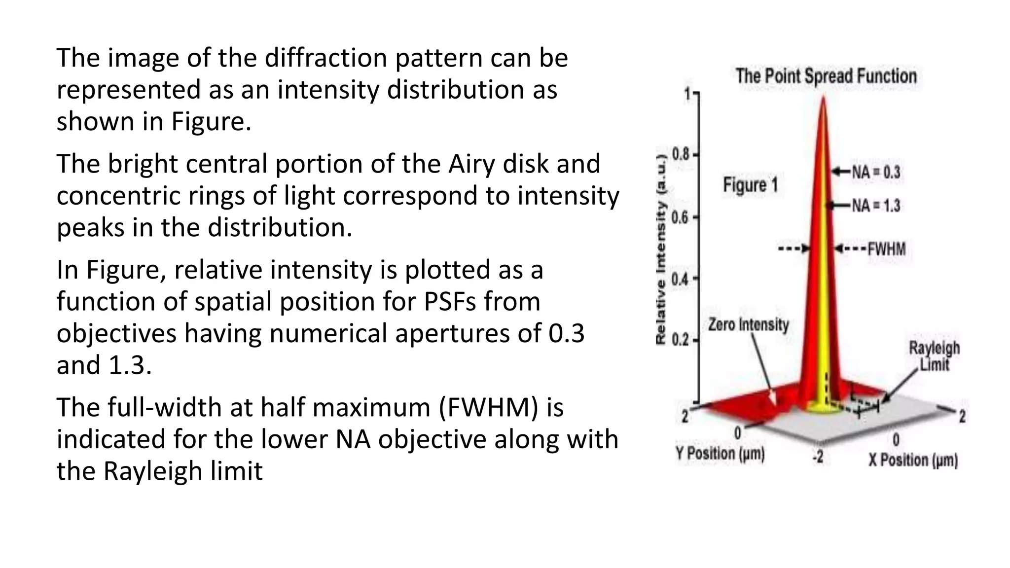
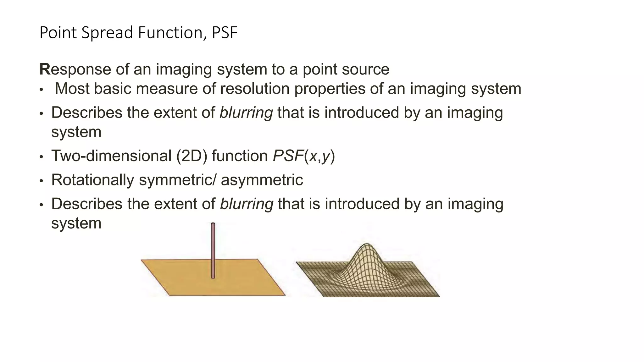
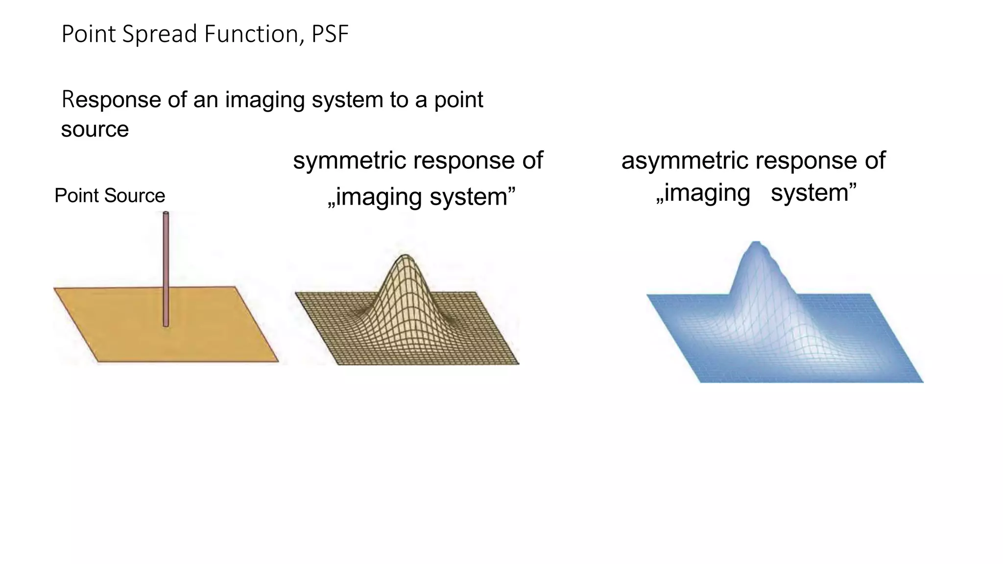
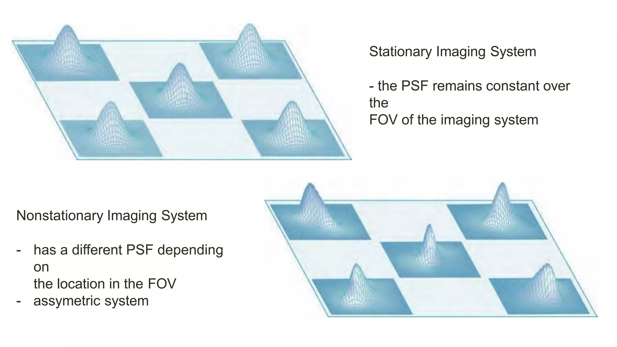
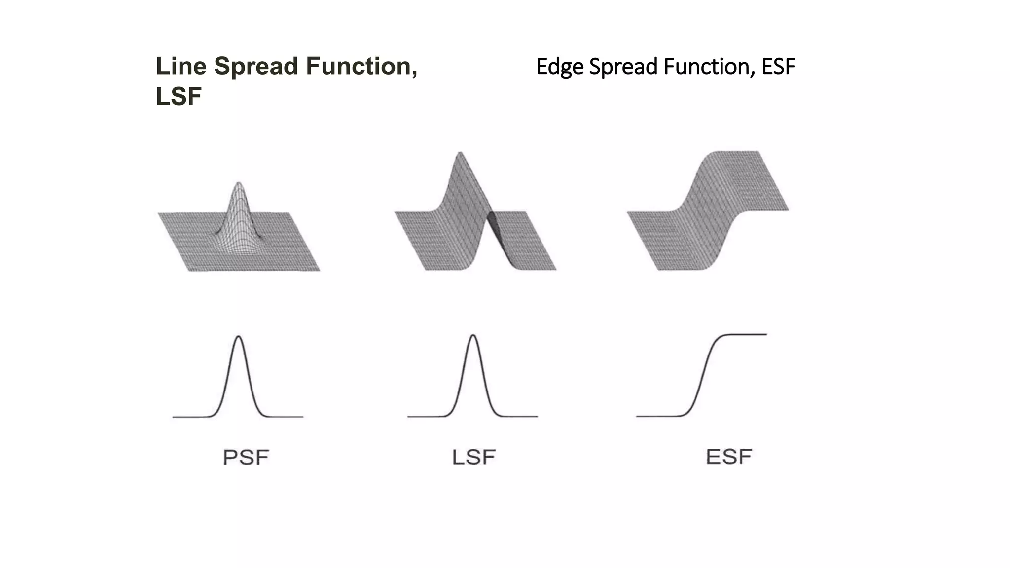
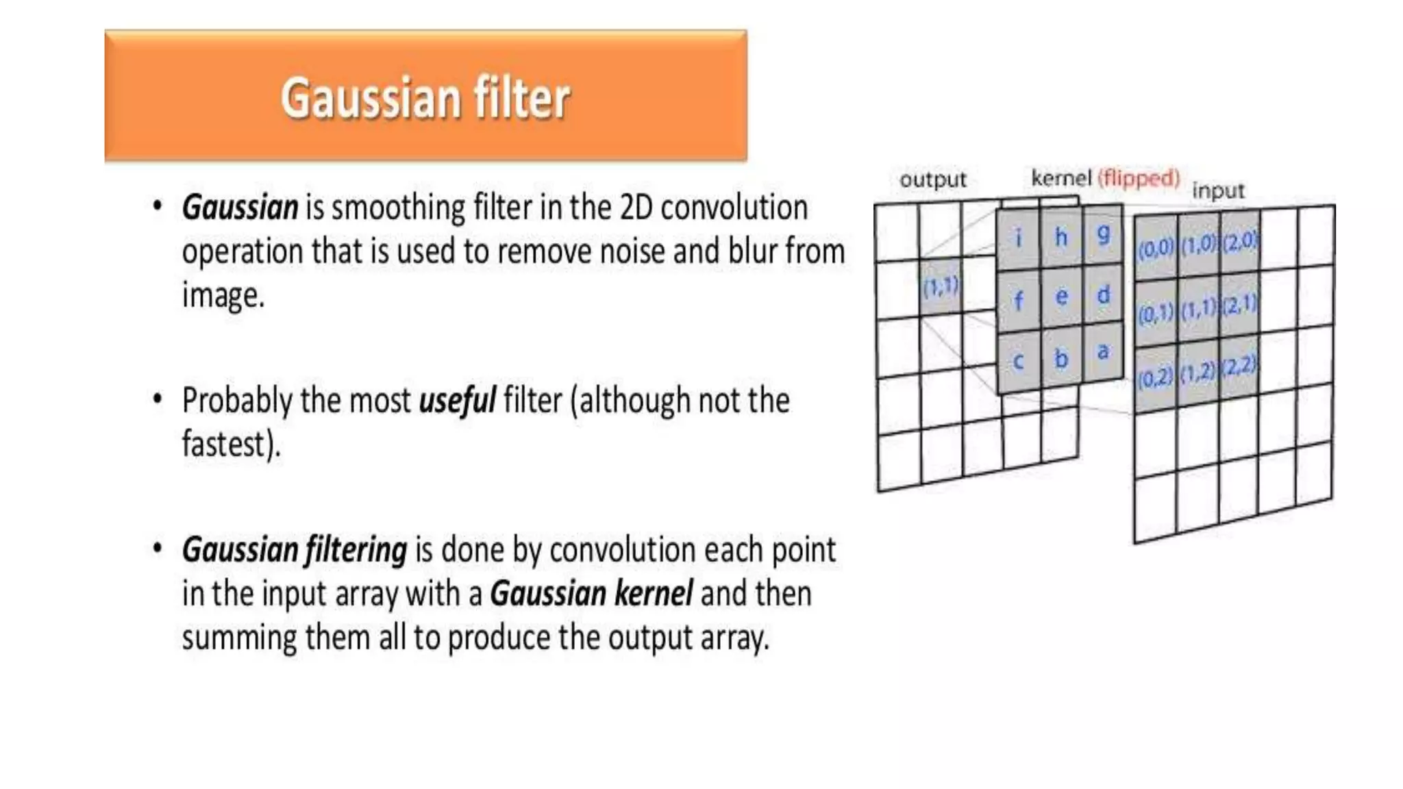
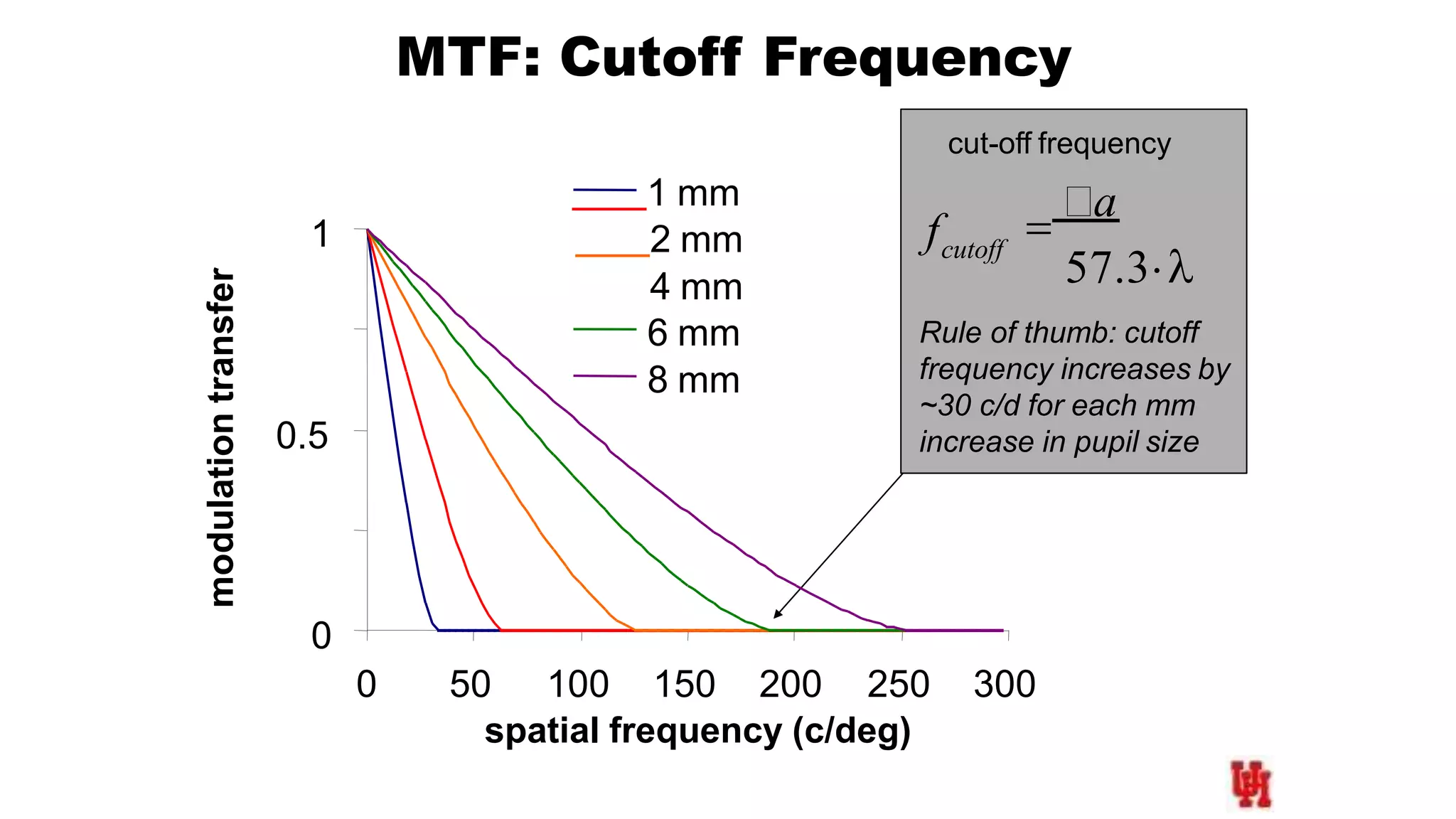
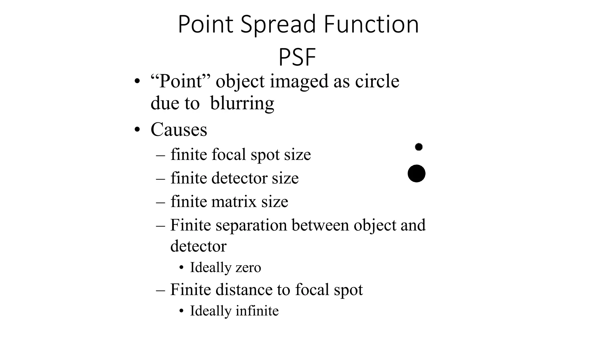
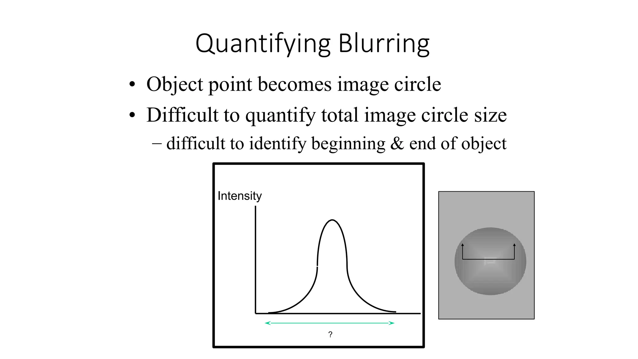
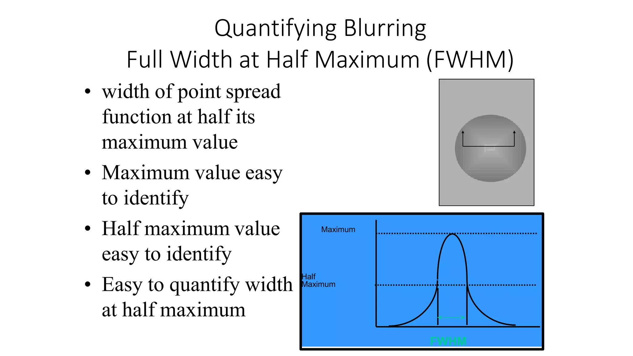
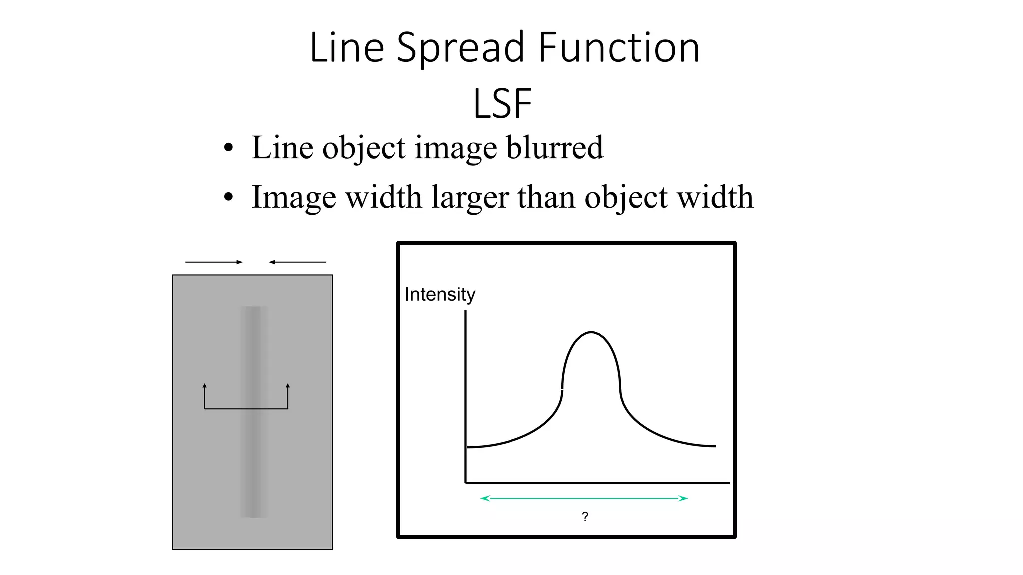
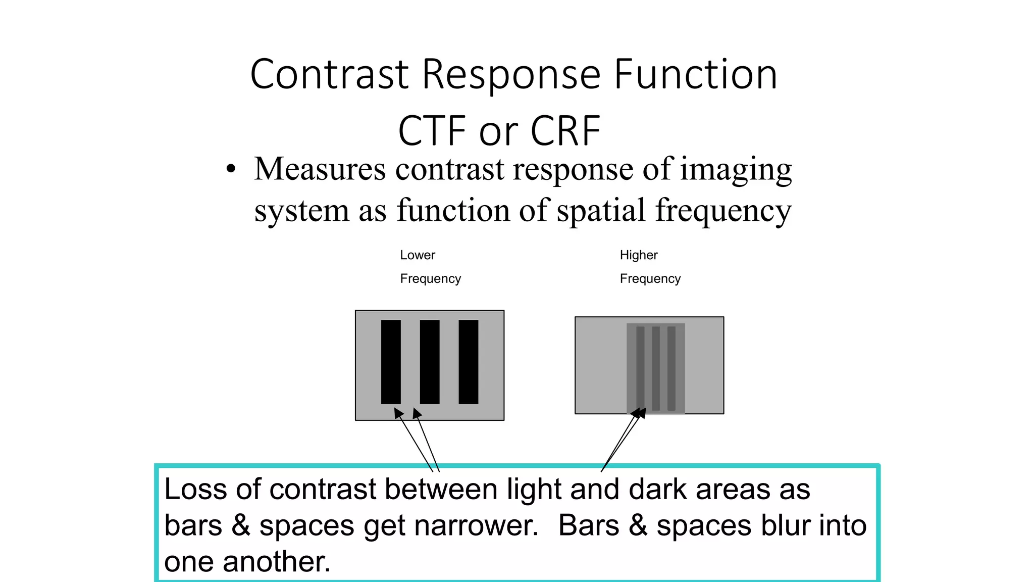
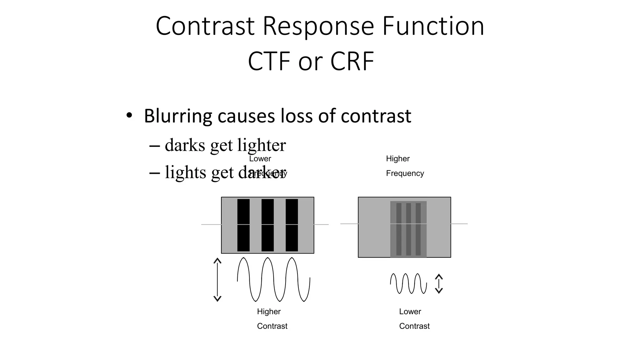
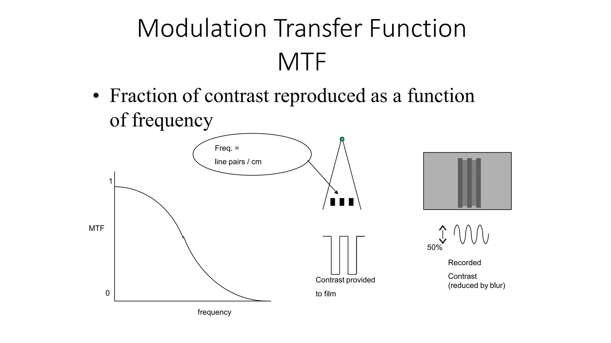
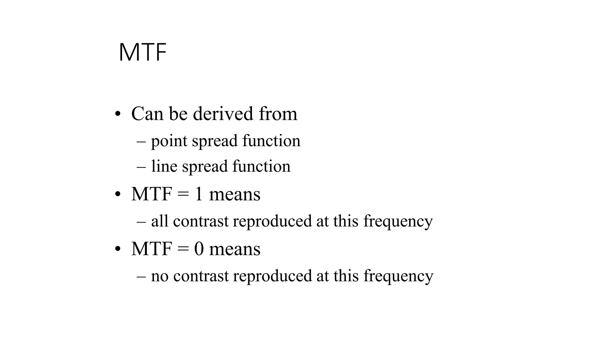
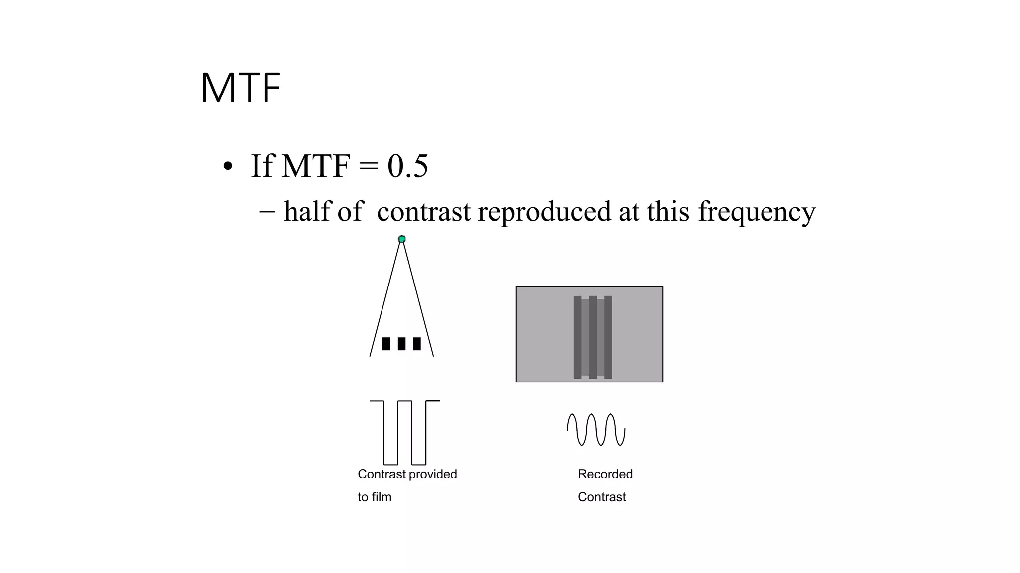
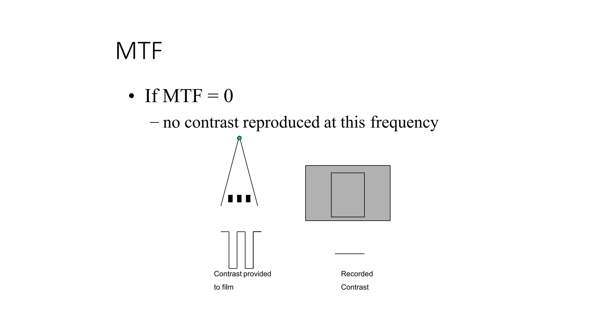
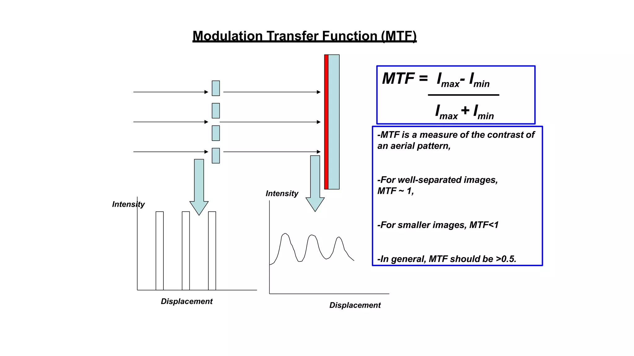
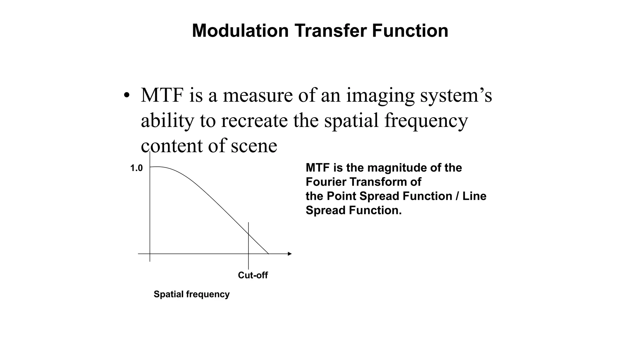
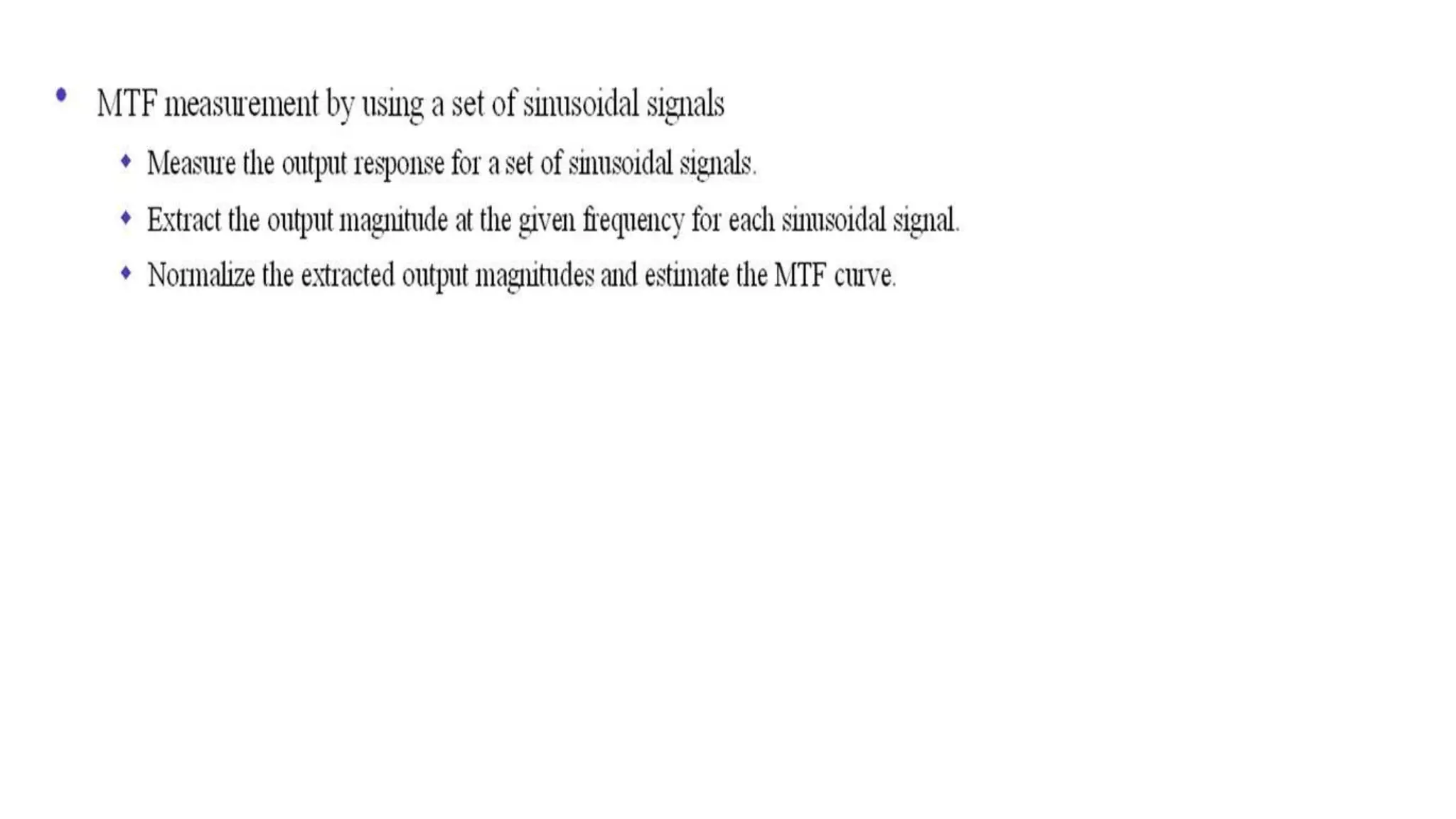
3. Radiographic Contrast
• Radiographic contrast is the degree of density difference
between two areas on a radiograph.
• Contrast makes it easier to distinguish features of interest, such
as defects, from the surrounding area.
• The image to the right shows two radiographs of the same
stepwedge.
• The upper radiograph has a high level of contrast and the lower
radiograph has a lower level of contrast.
• While they are both imaging the same change in thickness, the
high contrast image uses a larger change in radiographic density
to show this change.
• In each of the two radiographs, there is a small circle, which is
of equal density in both radiographs
4.
5. Radiographic Quality
Radiographic Quality refers to the fidelity with which the anatomic structures
being examined are imaged on the film.
Three mainfactors:
Film Factors
Geometric Factors
Subject Factors
Characteristic of radiographicquality:
Spatial Resolution (Recorded Detail)
Contrast Resolution (Visibility of Detail)
Noise (Visibility of Detail)
Artifacts
6. Spatial Resolution
Resolution is the ability to image two separate objects and visually
distinguish one from the other.
Spatial Resolution is the ability to image small structures that have high
subject contrast such as bone-soft tissue interface.
When all of the factors are correct, conventional radiography has
excellent spatial resolution.
Contrast Resolution
Contrast resolution is the ability to distinguish structures with similar subject
contrast such as liver-spleen, fat-muscle.
Computed tomography and MRIhave excellent contrast resolution.
Conventional radiography is fair to poor.
7. Noise
Noise is an undesirable fluctuationin optical density of the image.
Lower noise results in a better radiographic image because it improves contrast
resolution.
Two majortypes:
Film Graininess- no control over
Quantum Mottle- some control over
Film Graininess
Film graininess refers to thedistribution in size and space of the silver
halide grains in the film emulsion.
Similar to structure mottle that refers to the size and shape of the
phosphors in the intensifying screens.
Inherent in image receptor, and are not under the control of technologist,
and they contribute very little to radiographic noise.
8. Quantum Mottle
Quantum mottle refers to the random nature by which x-rays interact with the image
receptor.
Principal contributor to radiographic noise.
Image produced with few x rays will have higher QM than image produced with
from large number of x rays. use of very fast intensifying screens results in
increased QM.
The use of high mAs , low kVp settings and of slow image receptors reduces quantum
mottle.Very fast screens have higher quantum mottle because it takes fewer x-rays to
make the image.
Speed
Resolution and noise areintimately connected with speed.
While the speed of the images receptoris not apparent on the image, it
influences both resolution and noise.
9. Radiographic Quality Rules
• Fast Image receptors have high noiseand low spatial and contrast
resolution.
• High spatial and contrastresolution require low noise and
slow image receptors.
• Low noise accompanies slow image receptors with high spatial
and contrast resolution.
Film Factors of Quality
Characteristiccurve
Density
Contrast
Latitude
Processing
Time
Temperature
10. Sensitometry
• Sensitometry is the study of the relationship between the intensity of exposure
of the film and the blackness after the film is processed.
• Unexposed film is clear with a blue tint after processing.
• Properly exposed film appears with various shades of gray.
• Heavily Exposed film is blackafter processing.
Two principlesinvolved.
Exposure of the film
Amount of light transmitted through the
processed film of optical density.
Used to describe the relationship of radiation exposure and blackness or
optical density on the film.
11. Characteristic Curve
This relationship is called the characteristic
curve or H & D curve of the film.
H & D stands for Hurter and Driffield.
Parts of the Characteristic Curve
Toe and shoulder low and high , exposure
levels, where large changes in exposure results
in small changes in OD.
12. Parts of the Characteristic Curve
The straight line or intermediate area is
where very small changes in exposure
results in large changes in density.
This is the important part of the curve in
radiography,where properly exposed
radiographs appear.
13. Log Relative Exposure (LRE)
X-ray films responds to a wide range
of exposure from 1 mR to 1000 mR.
It is not the absolute exposure that is
of interest but rather the change in
OD over each exposure interval
Exposure is represented on
logarithmic manner(log relative
exposurer).
14. Optical Density
It is not enough to say that OD is the degree of blackening of a radiograph,or
that a clear area of the radiograph represent low OD and a black area represent
high OD.
OD density has a pre size numeric value that can be calculated if the level of light
incident on a processed film(Io)and the level of light transmitted through that film(It)
are measured.
OD=log10 Io/It
Optical Density Range
The optical density range is from 0.0 to
4.0 corresponding to clear and absolute black repectively.
Useful range in general radiography is from 0.5 to 2.25.
Image range is 0.5 to
1.25 OD
15. Fog density and base density
Most unexposed and processed film has an OD in the range of 0.1 to 0.3,corresponding to
79% and 50% transmission, respectively.these ODs of unexposed film are due to base
density and fog density.
Base density is inherent in the base of the film and is due to the composite of the base and
s the tint added to the base.
Fog density results from development of silver grains that
contain no useful information. Higher fog density reduces the
contrast of the image.
The tint of the base of the film and the inadvertent exposure of
the during processing.
Range is from 0.1 to 0.3. Should be never above 0.30 most is
0.21 OD
16. Things may Impact Base Fog
Filmstorage
Film exposure to wrong spectrum oflight or light intensity.
Chemicalcontamination.
Improperprocessing.
High Base fog levels reducecontrast.
Contrast
The variations in the OD in the radiograph is called radiographic contrast.
Marked differences in OD----High contrast radiograph.
OD differences are small----Low contrast radiograph
Radiographic Contrast is thecombined result of image receptor contrast and
subject contrast.
Image receptor contrast refers to the contrast inherent in the film and influenced
by the processing of the film.
17. Contrast
Subject contrast is determined by thesize, shape and x-ray attenuating
characteristics of the subject being examined and the energy (kVp) of the x- ray
beam.
Image Receptor Contrast
Inherent to the film and screen combination but is influenced by:
Range of Optical Density
Film Processing Technique
Film type is determined by the typeof intensifying screens used.
Film-screen images always have higher contrast compared with direct exposure
images.
18. Image Receptor Contrast
The slope of the straight line portion of the H & D
curve is the receptor contrast.
The average gradient is a straight line drawn
between the densities of 0.25 and 2.00 + base
fog.
Average Gradient
The average gradient is a straight line drawn
between
0.25 OD and 2.0 OD above base plus fog.
This is the useful range of optical density in
19. Speed
Speed is the ability of the receptor to respond to
low x-ray exposure.
The H & D curve is useful in comparing speed
when selecting film or screens.
A relative number of 100 given toPar Speed Calcium
Tungstate Screens.
High Speed Calcium Tungstate hasa speed of 200. Half
of the exposure is needed to produce the same image.
Rare earth screen filmcombinations range is speed from
80 to 1600.
20. LATITUDE
Latitude can be observed on the H & D curve.
Latitude refers to the range of exposure that
will produce a diagnostic range OD.
Latitude and Contrast are inversely
proportional.
Wide latitude has awide gray scale or low
contrast. (B)
Narrow latitude has a short scale or high
contrast. (A)
Latitude is designed into some screenand film combinations. With wide
latitude, the error factor in technique is wider.
Latitude can also be impacted bythe technical factors
21. Film Processing
Radiographic Quality is impacted by film
processing parameters.
The developer must be at the proper
concentration and at the correct temperature.
The film must also spend the correct amount of
time in the developer.
This is the time &temperature relationship.
22. Numerical Aperture (NA)
the numerical aperture (NA) of an optical system is a dimensionless
number that characterizes the range of angles over which the system
can accept or emit light. By incorporating index of refraction in its
definition, NA has the property that it is constant for a beam as it goes
from one material to another, provided there is no refractive power at
the interface.
23. Point Spread Function (PSF)
The ideal point spread function (PSF) is the three-dimensional diffraction pattern of
light emitted from an infinitely small point source in the specimen and transmitted to
the image plane through a high numerical aperture (NA) objective.
It is considered to be the fundamental unit of an image in theoretical models of image
formation.
When light is emitted from such a point object, a fraction of it is collected by the
objective and focused at a corresponding point in the image plane.
However, the objective lens does not focus the emitted light to an infinitely small point
in the image plane.
Rather, light waves converge and interfere at the focal point to produce a diffraction
pattern of concentric rings of light surrounding a central, bright disk, when viewed in
the x-y plane.
The radius of disk is determined by the NA, thus the resolving power of an objective
lens can be evaluated by measuring the size of the Airy disk (named after George
Biddell Airy).
24. The image of the diffraction pattern can be
represented as an intensity distribution as
shown in Figure.
The bright central portion of the Airy disk and
concentric rings of light correspond to intensity
peaks in the distribution.
In Figure, relative intensity is plotted as a
function of spatial position for PSFs from
objectives having numerical apertures of 0.3
and 1.3.
The full-width at half maximum (FWHM) is
indicated for the lower NA objective along with
the Rayleigh limit
25. Point Spread Function, PSF
Response of an imaging system to a point source
• Most basic measure of resolution properties of an imaging system
• Describes the extent of blurring that is introduced by an imaging
system
• Two-dimensional (2D) function PSF(x,y)
• Rotationally symmetric/ asymmetric
• Describes the extent of blurring that is introduced by an imaging
system
26. Point Spread Function, PSF
Response of an imaging system to a point
source
Point Source
symmetric response of
„imaging system”
asymmetric response of
„imaging system”
27. Stationary Imaging System
- the PSF remains constant over
the
FOV of the imaging system
Nonstationary Imaging System
- has a different PSF depending
on
the location in the FOV
- assymetric system
31. Modular Transfer Function
• The Modulation Transfer Function (MTF) is a method of determining the
response of an imaging system to different spatial frequencies in the
images.
• Spatial frequency is generally expressed as cycles, or line pairs, per
millimeter (lp/mm) in analog environments, but for digital systems,
cycles per pixel (c/p) is more appropriate where sensor sizes vary from
one detector to another.
• Two important parameters for determining the image quality in spatial
domain are contrast and resolution.
• MTF is an equivalent term which is used to characterize the image in
frequency domain.
• Generally, MTF for an imaging system is plotted as % amplitude against
spatial frequency.
32. • At frequencies where the MTF of an imaging system is 100%, the
object details are unattenuated and the image retains its full contrast.
Similarly, at a MTF of 50%, the contrast of the imaging system is
reduced by half of the original value.
• In imaging science, the MTF is usually normalized to 100% at very low
frequencies.
• The focal spot of the radiographic unit is one of the most important
parameters, because it influences the resolution of the image.
• There is a direct relationship between the focal spot and the MTF
curve of a radiography system. For large focal spot x-ray machines,
MTF values reach a minimum (i.e. zero) at comparative low spatial
frequency and vice versa.
33. Here, d1 is the source-to-object distance and d2 is the object-to-film distance. The parameter “f” equals the
spatial frequency of the sinusoidal object. The above equation is similar to an optical system because Fourier
transformation of a slit with width ‘a’ is (sin πfa / πfa). The value of MTF function will be zero where frequency
is such that the argument of sine function is equal to π or its multiples. If frequency is ‘f0’, for the MTF to be
zero,
The above equation shows that the maximum spatial frequency of the object (f0) (i.e. the finest details of the
object) is inversely proportional to the proportional focal spot size of the x-ray machine. MTF has a
multiplicative property. In radiography, the effective MTF is the multiplication of the MTF of film and that of
the focal spot.
Therefore, MTF(effective) = MTF(film) x MTF(focal spot)
34. • THE LINE spread-function (LSF) and modulation transfer function (MTF) of a screen-film
system convey important information regarding the light diffusion in the system, One of
the parameters influencing overall image quality.
• The LSF of a screen-film system is the relative illuminance distribution in the image of a
narrow slit.
• Thus, the LSF is a direct measure of light diffusion in screens and film.
• The MTF is a measure of the ability of the systems to image, frequency for frequency, a
radiation pattern in which intensity varies sinusoidally with distance in one dimension in
the object plane.
• The LSF and MTF of screen—film systems are parameters that can be used as a measure
of the image deterioration due to light diffusion only.
• The effect on image quality of other system characteristics, such as film contrast and
absorption of x-ray quanta in the screens resulting in quantum mottle, is not measured by
the LSF and MTF. Thus, the LSF and MTF do not, in themselves, provide a measure of the
overall image quality attainable with a screen—film system.
• The LSF and MTF are essentially different means of expressing the effect of light diffusion
in the screen—film system, and they are mathematically related (Fourier transform pair)
so that when one has been measured, the other can be calculated.
Note- This may vary system to system because its dependency on system
35. In Short
The resolution and performance of an optical microscope can be characterized
by a quantity known as the modulation transfer function (MTF), which is a
measurement of the microscope's ability to transfer contrast from the specimen
to the intermediate image plane at a specific resolution.
• Computation of the modulation transfer function is a mechanism that is often
utilized by optical manufacturers to incorporate resolution and contrast data
into a single specification. The modulation transfer function (MTF) indicates
the ability of an optical system to reproduce (transfer) various levels of
detail (spatial frequencies) from the object to the image.
• Its units are the ratio of image contrast over the object contrast as a
function of spatial frequency.
• It is the optical contribution to the contrast sensitivity function (CSF).
36. MTF: Cutoff Frequency
0.5
1
1 mm
2 mm
4 mm
6 mm
8 mm
modulationtransfer
0
0 50 100 150 200 250 300
spatial frequency (c/deg)
cut-off frequency
cutofff
a
57.3
Rule of thumb: cutoff
frequency increases by
~30 c/d for each mm
increase in pupil size
37. Measurements ofImage Quality
• PSF = Point Spread Function
• LSF = Line Spread Function
• CTF = Contrast Transfer Function
• MTF = Modulation Traffic Function
38. Point Spread Function
PSF
• “Point” object imaged as circle
due to blurring
• Causes
– finite focal spot size
– finite detector size
– finite matrix size
– Finite separation between object and
detector
• Ideally zero
– Finite distance to focal spot
• Ideally infinite
39. Quantifying Blurring
• Object point becomes image circle
• Difficult to quantify total image circle size
– difficult to identify beginning & end of object
Intensity
?
40. Quantifying Blurring
Full Width at Half Maximum (FWHM)
• width of point spread
function at half its
maximum value
• Maximum value easy
to identify
• Half maximum value
easy to identify
• Easy to quantify width
at half maximum
Maximum
Half
Maximum
FWHM
42. Contrast Response Function
CTF or CRF
• Measures contrast response of imaging
system as function of spatial frequency
Lower
Frequency
Higher
Frequency
Loss of contrast between light and dark areas as
bars & spaces get narrower. Bars & spaces blur into
one another.
43. Contrast Response Function
CTF or CRF
• Blurring causes loss of contrast
– darks get lighter
– lights get darker
Lower
Frequency
Higher
Frequency
Higher
Contrast
Lower
Contrast
45. MTF
• Can be derived from
– point spread function
– line spread function
• MTF = 1 means
– all contrast reproduced at this frequency
• MTF = 0 means
– no contrast reproduced at this frequency
46. MTF
• If MTF = 1
– all contrast reproduced at this frequency
Recorded
Contrast
Contrast provided
to film
47. MTF
• If MTF = 0.5
– half of contrast reproduced at this frequency
Recorded
Contrast
Contrast provided
to film
48. MTF
• If MTF = 0
– no contrast reproduced at this frequency
Recorded
Contrast
Contrast provided
to film
49. Modulation Transfer Function (MTF)
MTF = Imax- Imin
Imax + Imin
-MTF is a measure of the contrast of
an aerial pattern,
-For well-separated images,
MTF ~ 1,
-For smaller images, MTF<1
-In general, MTF should be >0.5.
Intensity
Intensity
DisplacementDisplacement
50. Component MTF
• Each component in an imaging system has its own
MTF
– each component retains a fraction of contrast as function
of frequency
• System MTF is product of MTF’s for each
component.
• Since MTF is between 0 and 1,
• composite MTF <= MTF of poorest component
51. Modulation Transfer Function
• MTF is a measure of an imaging system’s
ability to recreate the spatial frequency
content of scene
MTF is the magnitude of the
Fourier Transform of
the Point Spread Function / Line
Spread Function.
1.0
Cut-off
Spatial frequency