Introduction to Artificial Neural Networks

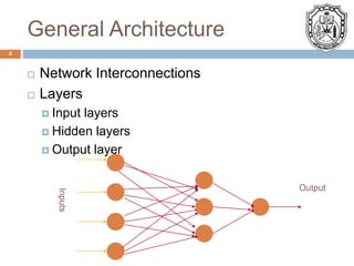
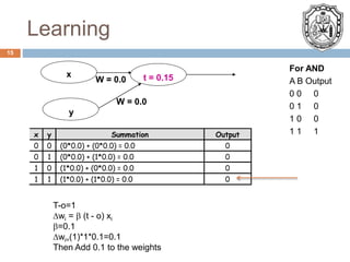
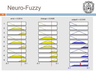
1. ARTIFICIAL NEURAL NETWORKS
End of Semester Presentation
Presented by:
Saif Al Kalbani 39579/12
20-05-2014
ECCE6206
Switching Theory: Design and
Practice
Spring 2014
1
Sultan Qaboos University
College of Engineering
Department of Electrical and
Computer Engineering

2. Outline
2
 Introduction
 General Architecture
 Learning
 Examples
 Applications
 Neuro-Fuzzy
 Conclusion

3. Applications
3
 Input is high-dimensional discrete or real-
valued (e.g. raw sensor input)
 Output is discrete or real valued
 Output is a vector of values
 Form of target function is unknown
 Control System
 Transfer function with huge number of inputs
 Unknown transfer function

4. General Architecture
4
 Network Interconnections
 Layers
 Input layers
 Hidden layers
 Output layer
Inputs
Output

5. General Architecture
5

6. General Architecture
6
 Threshold switching units
 Weighted interconnections among units
 Highly parallel, distributed processing
 Learning by tuning the connection weights

7. General Architecture
7

8. General Architecture
8
• Layers
• Activation function
• Learning

9. Layers
9
• The input layer.
– Introduces input values into the network.
– No activation function or other processing.
• The hidden layer(s).
– Perform classification of features
– Two hidden layers are sufficient to solve any problem
– Features imply more layers may be better
• The output layer.
– Functionally just like the hidden layers
– Outputs are passed on to the world outside the
neural network.

10. Examples
10

11. Activation Function
11

12. Learning
12
• Adjust neural network weights to map inputs to
outputs.
• Use a set of sample patterns where the desired
output (given the inputs presented) is known.
• The purpose is to learn to generalize
– Recognize features which are common to
good and bad exemplars
– Types
– Supervises
– Unsupervised

13. Supervised Learning
13
 Training and test data sets
 Training set; input & target

14. Learning
14
 wi = wi + wi
 wi =  (t - o) xi
 t=c(x) is the target value
 o is the perceptron output
  Is a small constant (e.g. 0.1) called learning rate
• If the output is correct (t=o) the weights wi are not
changed
• If the output is incorrect (to) the weights wi are
changed such that the output of the perceptron
for the new weights is closer to t.
 The algorithm converges to the correct
classification
• if the training data is linearly separable and  is
sufficiently small

15. Learning
15
For AND
A B Output
0 0 0
0 1 0
1 0 0
1 1 1
t = 0.15
y
x
W = 0.0
W = 0.0
x y Summation Output
0 0 (0*0.0) + (0*0.0) = 0.0 0
0 1 (0*0.0) + (1*0.0) = 0.0 0
1 0 (1*0.0) + (0*0.0) = 0.0 0
1 1 (1*0.0) + (1*0.0) = 0.0 0
T-o=1
wi =  (t - o) xi
=0.1
wi=(1)*1*0.1=0.1
Then Add 0.1 to the weights

16. Learning
16
For AND
A B Output
0 0 0
0 1 0
1 0 0
1 1 1
t = 0.15
y
x
W = 0.1
W = 0.1
x y Summation Output
0 0 (0*0.1) + (0*0.1) = 0.0 0
0 1 (0*0.1) + (1*0.1) = 0.1 0
1 0 (1*0.1) + (0*0.1) = 0.1 0
1 1 (1*0.1) + (1*0.1) = 0.2 1

17. Decision Boundary
17
X1
X2
A
B
A
A
A
A
A
A
B
B
B
B
B
B
B Decision
Boundary

18. Strength
18
 Solving complex problems
 Inputs are complex, large, unknown
 Transfer function is unknown
 Adaptation
 Adaptive controllers
 Learning process

19. Shortfalls
19
 Learning
 Weights
 Processing time
 Delays in processing
 Sensing
 Set up
 Layers

20. Application Example
20
• Engine Control Unit (ECU) in new cars
• Fuel injector
• The behaviour of a car engine is influenced by a
large number of parameters
– temperature at various points
– fuel/air mixture
– lubricant viscosity.
• Major companies have used neural networks to
dynamically tune an engine depending on
current settings.

21. Neuro-Fuzzy
21
 Hybrid controllers
 ANN controllers
 Fuzzy logic Controllers
 Adaptation
 Rules
 Membership functions

22. Neuro-Fuzzy
22

23. Conclusion
23
 Ability of ANN to
 Adapt through learning
 Solve complex systems
 ANN is claimed to be able to solve any
problem with a maximum of two hidden layers

24. Thank You
Q&A24

25. Back-up25

26. Fuzzy System
26