This document provides an overview of machine learning concepts for assessing model performance including metrics, model selection, and diagnostics. It discusses classification and regression metrics like accuracy, precision, recall, ROC curves, and coefficients of determination. Model selection techniques covered are training/validation/test sets, cross-validation, and regularization. Diagnostics examines bias/variance tradeoffs and remedies for underfitting and overfitting.

1. CS 229 – Machine Learning https://stanford.edu/~shervine
VIP Cheatsheet: Machine Learning Tips
Afshine Amidi and Shervine Amidi
September 9, 2018
Metrics
Given a set of data points {x(1), ..., x(m)}, where each x(i) has n features, associated to a set of
outcomes {y(1), ..., y(m)}, we want to assess a given classifier that learns how to predict y from
x.
Classification
In a context of a binary classification, here are the main metrics that are important to track to
assess the performance of the model.
r Confusion matrix – The confusion matrix is used to have a more complete picture when
assessing the performance of a model. It is defined as follows:
Predicted class
+ –
Actual class
TP FN
+ False Negatives
True Positives
Type II error
FP TN
– False Positives
True Negatives
Type I error
r Main metrics – The following metrics are commonly used to assess the performance of
classification models:
Metric Formula Interpretation
Accuracy
TP + TN
TP + TN + FP + FN
Overall performance of model
Precision
TP
TP + FP
How accurate the positive predictions are
Recall
TP
TP + FN
Coverage of actual positive sample
Sensitivity
Specificity
TN
TN + FP
Coverage of actual negative sample
F1 score
2TP
2TP + FP + FN
Hybrid metric useful for unbalanced classes
r ROC – The receiver operating curve, also noted ROC, is the plot of TPR versus FPR by
varying the threshold. These metrics are are summed up in the table below:
Metric Formula Equivalent
True Positive Rate
TP
TP + FN
Recall, sensitivity
TPR
False Positive Rate
FP
TN + FP
1-specificity
FPR
r AUC – The area under the receiving operating curve, also noted AUC or AUROC, is the
area below the ROC as shown in the following figure:
Regression
r Basic metrics – Given a regression model f, the following metrics are commonly used to
assess the performance of the model:
Total sum of squares Explained sum of squares Residual sum of squares
SStot =
m
X
i=1
(yi − y)2
SSreg =
m
X
i=1
(f(xi) − y)2
SSres =
m
X
i=1
(yi − f(xi))2
r Coefficient of determination – The coefficient of determination, often noted R2 or r2,
provides a measure of how well the observed outcomes are replicated by the model and is defined
as follows:
R2
= 1 −
SSres
SStot
r Main metrics – The following metrics are commonly used to assess the performance of
regression models, by taking into account the number of variables n that they take into consid-
eration:
Mallow’s Cp AIC BIC Adjusted R2
SSres + 2(n + 1)b
σ2
m
2
(n + 2) − log(L)
log(m)(n + 2) − 2 log(L) 1 −
(1 − R2)(m − 1)
m − n − 1
Stanford University 1 Fall 2018

2. CS 229 – Machine Learning https://stanford.edu/~shervine
where L is the likelihood and b
σ2 is an estimate of the variance associated with each response.
Model selection
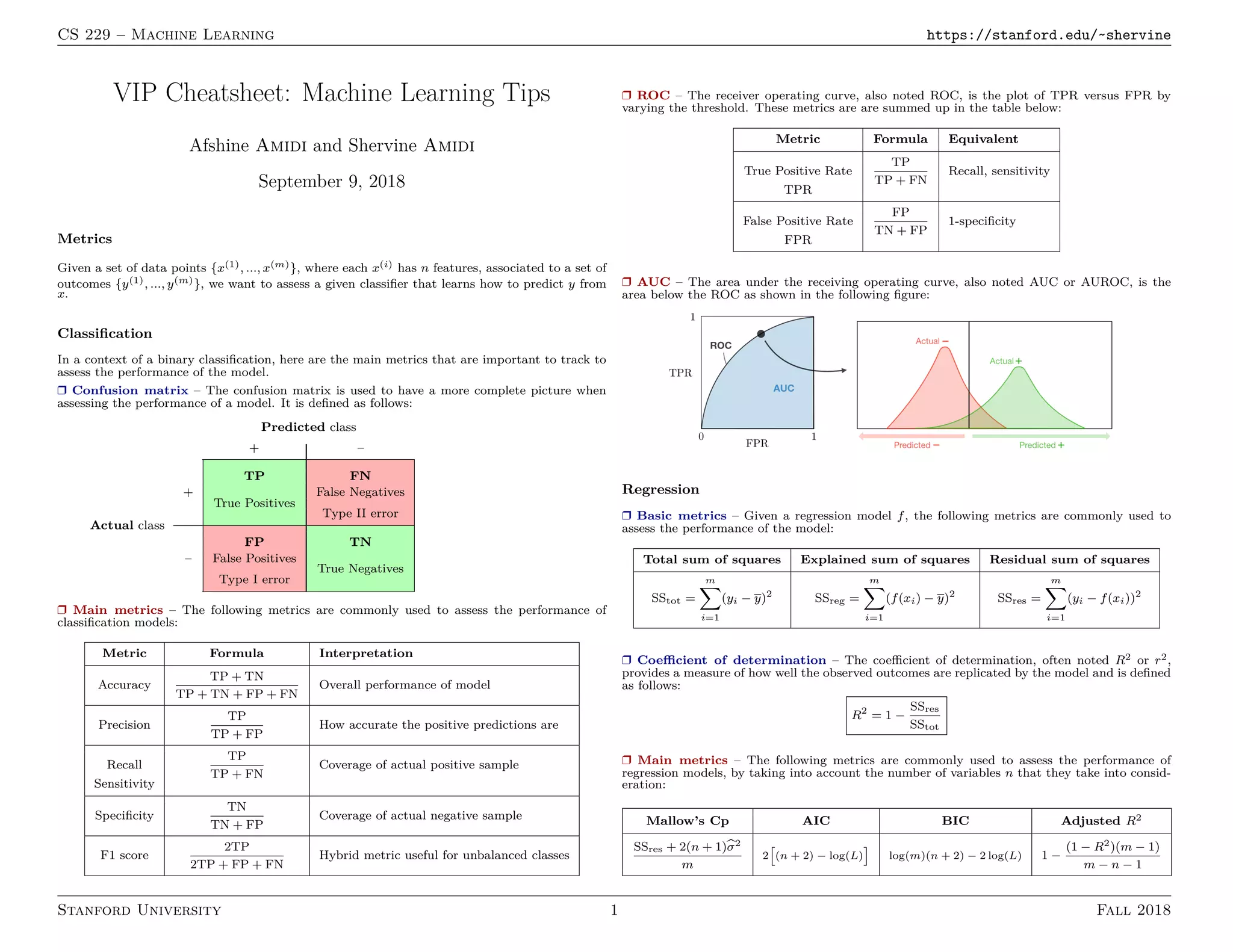
r Vocabulary – When selecting a model, we distinguish 3 different parts of the data that we
have as follows:
Training set Validation set Testing set
- Model is trained - Model is assessed - Model gives predictions
- Usually 80% of the dataset - Usually 20% of the dataset - Unseen data
- Also called hold-out
or development set
Once the model has been chosen, it is trained on the entire dataset and tested on the unseen
test set. These are represented in the figure below:
r Cross-validation – Cross-validation, also noted CV, is a method that is used to select a
model that does not rely too much on the initial training set. The different types are summed
up in the table below:
k-fold Leave-p-out
- Training on k − 1 folds and - Training on n − p observations and
assessment on the remaining one assessment on the p remaining ones
- Generally k = 5 or 10 - Case p = 1 is called leave-one-out
The most commonly used method is called k-fold cross-validation and splits the training data
into k folds to validate the model on one fold while training the model on the k − 1 other folds,
all of this k times. The error is then averaged over the k folds and is named cross-validation
error.
r Regularization – The regularization procedure aims at avoiding the model to overfit the
data and thus deals with high variance issues. The following table sums up the different types
of commonly used regularization techniques:
LASSO Ridge Elastic Net
- Shrinks coefficients to 0 Makes coefficients smaller Tradeoff between variable
- Good for variable selection selection and small coefficients
... + λ||θ||1 ... + λ||θ||2
2 ... + λ
h
(1 − α)||θ||1 + α||θ||2
2
i
λ ∈ R λ ∈ R λ ∈ R, α ∈ [0,1]
r Model selection – Train model on training set, then evaluate on the development set, then
pick best performance model on the development set, and retrain all of that model on the whole
training set.
Diagnostics
r Bias – The bias of a model is the difference between the expected prediction and the correct
model that we try to predict for given data points.
r Variance – The variance of a model is the variability of the model prediction for given data
points.
r Bias/variance tradeoff – The simpler the model, the higher the bias, and the more complex
the model, the higher the variance.
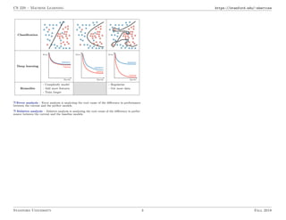
Underfitting Just right Overfitting
- High training error - Training error - Low training error
Symptoms - Training error close slightly lower than - Training error much
to test error test error lower than test error
- High bias - High variance
Regression
Stanford University 2 Fall 2018

3. CS 229 – Machine Learning https://stanford.edu/~shervine
Classification
Deep learning
- Complexify model - Regularize
Remedies - Add more features - Get more data
- Train longer
r Error analysis – Error analysis is analyzing the root cause of the difference in performance
between the current and the perfect models.
r Ablative analysis – Ablative analysis is analyzing the root cause of the difference in perfor-
mance between the current and the baseline models.
Stanford University 3 Fall 2018