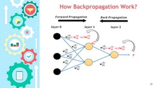
This document provides an outline for a course on neural networks and fuzzy systems. The course is divided into two parts, with the first 11 weeks covering neural networks topics like multi-layer feedforward networks, backpropagation, and gradient descent. The document explains that multi-layer networks are needed to solve nonlinear problems by dividing the problem space into smaller linear regions. It also provides notation for multi-layer networks and shows how backpropagation works to calculate weight updates for each layer.
Framing an Appropriate Research Question 6b9b26d93da94caf993c038d9efcdedb.pdf
Β
04 Multi-layer Feedforward Networks
1. Neural Networks and
Fuzzy Systems
Multi-layer Feed forward Networks
Dr. Tamer Ahmed Farrag
Course No.: 803522-3
2. Course Outline
Part I : Neural Networks (11 weeks)
β’ Introduction to Machine Learning
β’ Fundamental Concepts of Artificial Neural Networks
(ANN)
β’ Single layer Perception Classifier
β’ Multi-layer Feed forward Networks
β’ Single layer FeedBack Networks
β’ Unsupervised learning
Part II : Fuzzy Systems (4 weeks)
β’ Fuzzy set theory
β’ Fuzzy Systems
2
3. Outline
β’ Why we need Multi-layer Feed forward Networks
(MLFF)?
β’ Error Function (or Cost Function or Loss function)
β’ Gradient Descent
β’ Backpropagation
3
4. Why we need Multi-layer Feed forward
Networks (MLFF)?
β’ Overcoming failure of single layer perceptron in
solving nonlinear problems.
β’ First Suggestion:
β’ Divide the problem space into smaller linearly separable
regions
β’ Use a perceptron for each linearly separable region
β’ Combine the output of multiple hidden neurons to
produce a final decision neuron.
4
Region 1
Region 2
5. Why we need Multi-layer Feed forward
Networks (MLFF)?
β’ Second suggestion
β’ In some cases we need a curve decision boundary or we try to solve
more complicated classification and regression problems.
β’ So, we need to:
β’ Add more layers
β’ Increase a number of neurons in each layer.
β’ Use non linear activation function in
the hidden layers.
β’ So , we need Multi-layer Feed forward Networks (MLFF).
5
6. Notation for Multi-Layer Networks
β’ Dealing with multi-layer networks is easy if a sensible notation is adopted.
β’ We simply need another label (n) to tell us which layer in the network we
are dealing with.
β’ Each unit j in layer n receives activations ππ’π‘π
(πβ1)
π€ππ
(π)
from the previous
layer of processing units and sends activations ππ’π‘π
(π)
to the next layer of
units.
6
1
2
3
1
2
layer (0) layer (1)
πππ
(π)
layer (n-1) layer (n)
πππ
(π)
9. Error Function
β how we can evaluate performance of a neuron
????
β We can use a Error function (or cost function or
loss function) to measure how far off we are from
the expected value.
β Choosing appropriate Error function help the
learning algorithm to reach to best values for
weights and biases.
β Weβll use the following variables:
β D to represent the true value (desired value)
β y to represent neuronβs prediction 9
10. Error Functions
(Cost function or Lost Function)
β’ There are many formulates for error functions.
β’ In this course, we will deal with two Error function
formulas.
Sum Squared Error (SSE) :
π ππ = π¦π β π·π
2
for single perceptron
πΈπππΈ=
π=1
π
π¦π β π·π
2
1
Cross entropy (CE):
πΈ πΆπΈ =
1
π π=1
π
[π·π β ln(π¦π) + (1β π·π) β ln(1β π¦π)] (2)
10
1
2
11. Why the error in ANN occurs?
β’ Each weight and bias in the network contribute in
the occasion of the error.
β’ To solve this we need:
β’ A cost function or error function to compute the error.
(SSE or CE Error function)
β’ An optimization algorithm to minimize the error
function. (Gradient Decent)
β’ A learning algorithm to modify weights and biases to
new values to get the error down. (Backpropagation)
β’ Repeat this operation until find the best solution
11
12. Gradient Decent (in 1 dimension)
β’ Assume we have a error function E and we need to
use it to update one weight w
β’ The figure show the error function in terms of w
β’ Our target is to learn the value of w produces the
minimum value of E.
How?
12
E
W
minimum
13. Gradient Decent (in 1 dimension)
β’ In Gradient Decent algorithm, we use the following
equation to get a better value of w:
π€ = π€ β Ξ±Ξπ€ (called Delta rule)
Where:
Ξ± : is the learning rate
Ξπ€ : is mathematically can be computed using
derivative of E with respect to w (
ππΈ
ππ€
)
13
E
W
minimum
π€ = π€ β Ξ±
ππΈ
ππ€
(3)
16. Gradient Decent (multi dimension)
β’ In ANN with many layers and many neurons in each layer the
Error function will be multi-variable function.
β’ So, the derivative in equation (3) should be partial derivative
π€ππ = π€ππ β Ξ±
ππΈ π
ππ€ ππ
(4)
β’ We write equation (4) as :
π€ππ = π€ππ β Ξ± ππ€ππ
β’ Same process will be use to get the
new bias value:
ππ= ππ β Ξ± πππ
16
20. Learning Rule in the Hidden layer
β’ Now we have to determine the appropriate
weight change for an input to hidden weight.
β’ This is more complicated because it depends on
the error at all of the nodes this weighted
connection can lead to.
β’ The mathematical proof is out our scope.
20
21. Gradient Decent (Notes)
Note 1:
β’ the neuron activation function (f ) should be is defined
and differentiable function.
Note 3:
β’ The calculating of ππ€ππ for the hidden layer will be
more difficult (Why?)
Note 2:
β’ The previous calculation will be repeated for each
weight and for each bias in the ANN
β’ So, we need big computational power (what about
deeper networks? )
21
22. Gradient Decent (Notes)
β’ ππ€ππ is represent the change in the values of π€ππ
to get better output
β’ The equation of ππ€ππ is dependent on the choosing
of the Error(Cost) function and activation function.
β’ Gradient Decent algorithm help in calculated the
new values of weights and bias.
β’ Question: is one iteration (one trail) enough to
bet the best values for weights and biases
β’ Answer: No, we need a extended version ?
Backpropagation
22
24. Online Learning vs. Offline Learning
β’ Online: Pattern-by-Pattern
learning
β’ Error calculated for each
pattern
β’ Weights updated after each
individual pattern
π«πππ = βπΆ
ππ¬ π
ππππ
β’ Offline: Batch learning
β’ Error calculated for all
patterns
β’ Weights updated once at
the end of each epoch
π«πππ = βπΆ
π
ππ¬ π
ππππ
24
25. Choosing Appropriate Activation and Cost
Functions
β’ We already know consideration of single layer networks what
output activation and cost functions should be used for
particular problem types.
β’ We have also seen that non-linear hidden unit activations are
needed, such as sigmoids.
β’ So we can summarize the required network properties:
β’ Regression/ Function Approximation Problems
β’ SSE cost function, linear output activations, sigmoid hidden activations
β’ Classification Problems (2 classes, 1 output)
β’ CE cost function, sigmoid output and hidden activations
β’ Classification Problems (multiple-classes, 1 output per class)
β’ CE cost function, softmax outputs, sigmoid hidden activations
β’ In each case, application of the gradient descent learning
algorithm (by computing the partial derivatives) leads to
appropriate back-propagation weight update equations.
25
27. Neural network simulator
β’ Search through the internet to find a simulator and
report it
For example:
β’ https://www.mladdict.com/neural-network-
simulator
β’ http://playground.tensorflow.org/
27