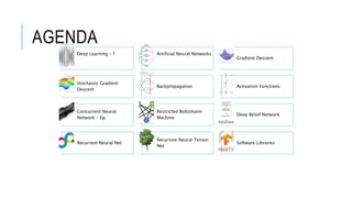
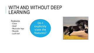
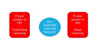
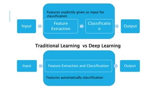
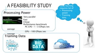
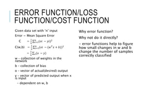
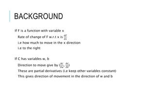
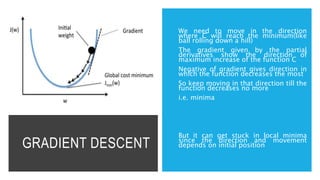
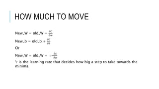
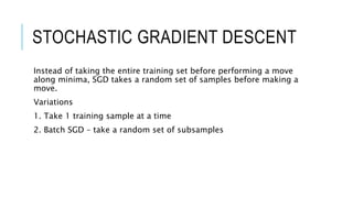
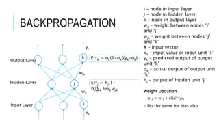
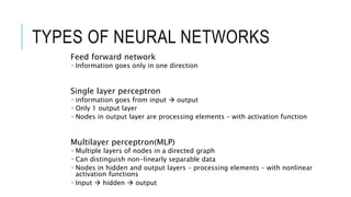
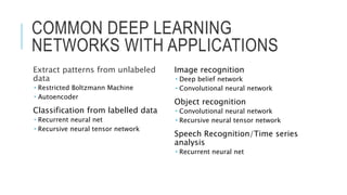
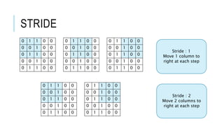
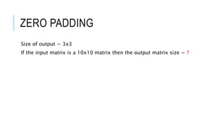
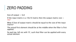
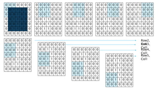
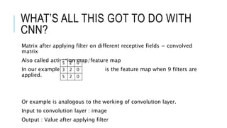
DEEP LEARNING
Dr.S.Lovelyn Rose
Associate Professor
Dept. of CSE
PSG CT, Cbe.
AGENDA
Deep Learning – ? Artificial Neural Networks
Gradient Descent
Stochastic Gradient
Descent
Backpropagation Activation Functions
Concurrent Neural
Network – Eg.
Restricted Boltzmann
Machine
Deep Belief Network
Recurrent Neural Net
Recursive Neural Tensor
Net
Software Libraries
WITH AND WITHOUT DEEP
LEARNING
Features
 Crest
 Hoof
 Muscular legs
 Muzzle
 Lush tail
Do I
explicitly
state the
features?
Do I
explicitly
state the
features?
If your
answer is
NO
Deep
Learning
If your
answer is
YES
Traditional
Learning
Input
Feature
Extraction
Classificatio
n
Output
Input Feature Extraction and Classification Output
Traditional Learning vs Deep Learning
Features explicitly given as input for
classification
Features automatically classification
Processing Power
Very parallel
Fast
Cheap
Performance benchmark
PC CPU – 1 -3 Gflops/sec
average
GPU – 100 Gflops/sec
average
A FEASIBILITY STUDY Deep learning
requires lot of
• Processing
power
• Training
data
Training Data
ARTIFICIAL NEURAL
NETWORKS
MCCULLOCH AND PITTS NETWORK
Linear threshold gate
Input : x1, x2, … xn
Output : Y – binary
Weights : w1, w2, … wn
Weights Normalized : (0,1), (-0.5,0.5), (-1,1)
Calculate Net Input : I = 𝑘=1
𝑛
𝑥 𝑘 ∗ 𝑤𝑘
Activation Function = f(I) =
1, 𝑖𝑓 𝐼 ≥ 𝑇
0, 𝑖𝑓 𝐼 < 𝑇
- binary step function
Σ
xn
x2
x1
…
w1
w2
wn
ACTIVATION FUNCTIONS
Heaviside Step function
Output either 0 or 1
𝑓 𝐼 =
0, 𝐼 < 0
1, 𝐼 ≥ 0
Linear function
 Input is the output
 𝑓 𝐼 =I
Sign function
 Output either -1 or 1
 𝑓 𝐼 =
−1, 𝐼 < 0
1, 𝐼 ≥ 0
SIGMOID FUNCTION
Sigmoid Function
 Mathematical function with S shaped curve(sigmoid curve)
Types of Sigmoid functions
Logistic function
 Output between 0 and 1
 f(I) =
1
1+𝑒−𝐼
Hyperbolic tangent
 Output between -1 and 1
 f(I) =
𝑒2𝐼−1
𝑒2𝐼+1
RECTIFIED LINEAR UNIT (RELU)[
Commonly used in deep learning
Empirically good result
LINEARLY SEPARABLE
X Y X AND Y
1 1 1
1 0 0
0 1 0
0 0 0
0
0.2
0.4
0.6
0.8
1
1.2
0 0.5 1 1.5
AND Function
X Y X OR Y
1 1 1
1 0 1
0 1 1
0 0 0
0
0.2
0.4
0.6
0.8
1
1.2
0 0.5 1 1.5
OR Function
X Y X XOR Y
1 1 0
1 0 1
0 1 1
0 0 1
0
0.2
0.4
0.6
0.8
1
1.2
0 0.5 1 1.5
XOR Function
Right of line : Output
should fire
EXAMPLE – AND FUNCTION
Let wi = 1 ∀ i
Net input (1,1) : 1*1+ 1*1 = 2
Net input (1,0) : 1*1+ 0*1 = 1
Net input (0,1) : 0*1+ 1*1 = 1
Net input (0,0) : 0*1+ 0*1 = 0
Set T = 2
 Output : 1, if T ≥ 2
 Output : 0, if T < 2
Remember we designed the network
X
Y
X AND
Y
w1
w2
QUESTION TIME
What changes do you need to make to implement an OR function
LINE – SOME MATHEMATICS
𝑦 = 𝑤0. 𝑥0 + 𝑤1. 𝑥1 + … + 𝑤 𝑛. 𝑥 𝑛
= 𝑖=1
𝑛
𝑤𝑖 𝑥𝑖
= 𝑤 𝑇 𝑥
INTRODUCING BIAS
Classifier tries to find line to separate classes
y=mx+c
In training phase neural network tries to learn appropriate weights to
draw the line
If there is no y intercept, any line we draw will pass through origin
So introduce y-intercept as bias
If we set the bias to 1 then why does it make difference to the fit now
that every line will now go through (0,1) instead of (0,0)
by multiplying a bias by a weight, you can shift it by an arbitrary
amount
BIAS AND THE SIGMOID FUNCTION
(x1,x2) = (0.2, 0.5)
(w0,w1,w2) = (0.4, 0.3, 0.5)
b = 1
Net input : I = 1*0.4 + 0.2*0.3 + 0.5*0.5
= 0.71
y =
1
1+ 𝑒−𝐼 =
1
1+ 𝑒−0.71 = 0.67
x1
x2
y
w1
w2
w0
b
PERCEPTRON
Binary classifier
Let input x = ( x1, x2, ... , xn) where each xi = 0 or 1.
And let output y = 0 or 1.
Algorithm is repeat forever:
 Given input x = ( x1, x2, ... , xn).
 Perceptron produces output y.
 The correct output is O.
 If we had wrong answer, change wi's and T, otherwise do nothing.
Single layer perceptron solves only linearly separable problems
HOW TO CHANGE wi
y – Predicted output – 0.67
O – Actual output – 1
Change wi based on (O-y)
Use error function to connect actual and predicted output
ERROR FUNCTION/LOSS
FUNCTION/COST FUNCTION
Given data set with ‘n’ input
Error = Mean Square Error
C =
1
𝑛 𝑖=1
𝑛
(𝑜𝑖 − 𝑦𝑖)2
C(w,b) =
1
𝑛 𝑖=1
𝑛
(𝑜𝑖 − (𝑤 𝑇
𝑥 + 𝑏))2
=
1
𝑛 𝑥(𝑜 − 𝑦)
w – collection of weights in the
network
b – collection of bias
o – vector of actual(desired) output
y – vector of predicted output when x
is input
- dependent on w, b
Why error function?
Why not do it directly?
- error functions help to figure
how small changes in w and b
change the number of samples
correctly classified
OBJECTIVE
- Minimize error function
- Minimize C(w,b)
- Perfect if the C(w,b) = 0
- Good if C(w,b) ≈ 0
- i.e Find weights and bias such that C(w,b) ≈ 0
- To do this use “Gradient Descent”
GRADIENT DESCENT
GRADIENT
Or slope
How steep is the line
What is the change in y when x
changes
Why not just
call it slope?
GRADIENT
- involves more than 2 parameters
– here w, b and C(w,b)
Gradient – Vector calculus
 Gives direction in which a given function increases the maximum
w
w
b
C(w,
b)
BACKGROUND
If F is a function with variable x
Rate of change of F w.r.t x is
𝑑𝐹
𝑑𝑥
i.e how much to move in the x direction
i.e to the right
If C has variables w, b
Direction to move give by (
𝜕𝐶
𝜕𝑤
,
𝜕𝐶
𝜕𝑏
)
These are partial derivatives (i.e keep other variables constant)
This gives direction of movement in the direction of w and b
GRADIENT DESCENT
We need to move in the direction
where C will reach the minimum(like
ball rolling down a hill)
The gradient given by the partial
derivatives show the direction of
maximum increase of the function C
Negative of gradient gives direction in
which the function decreases the most
So keep moving in that direction till the
function decreases no more
i.e. minima
But it can get stuck in local minima
since the direction and movement
depends on initial position
HOW MUCH TO MOVE
New_W = old_W +
𝜕𝐶
𝜕𝑤
New_b = old_b +
𝜕𝐶
𝜕𝑏
Or
New_W = old_W + l
𝜕𝐶
𝜕𝑤
‘l’ is the learning rate that decides how big a step to take towards the
minima
STOCHASTIC GRADIENT DESCENT
Instead of taking the entire training set before performing a move
along minima, SGD takes a random set of samples before making a
move.
Variations
1. Take 1 training sample at a time
2. Batch SGD – take a random set of subsamples
BACKPROPAGATION
i
j
k
wij
wjk
Input Layer
Hidden Layer
Output Layer
yt
xs
i – node in input layer
j – node in hidden layer
k – node in output layer
wij – weight between nodes ‘i’
and ‘j’
wjk – weight between nodes ‘j’
and ‘k’
X – input vector
xs – input value of input unit ‘s’
yk – predicted output of output
unit ‘k’
ok – actual output of output unit
‘k’
hj – output of hidden unit ‘j’
Errk = ok(1-ok)(yk-ok)
Errj = hj(1-
hj) 𝑘 𝐸𝑟𝑟𝑘 𝑤𝑗𝑘
𝑤𝑖𝑗 = 𝑤𝑖𝑗 + (𝑙)𝐸𝑟𝑟𝑗 𝑜𝑖
Weight Updation
- Do the same for bias also
TYPES OF NEURAL NETWORKS
Feed forward network
 Information goes only in one direction
Single layer perceptron
 information goes from input  output
 Only 1 output layer
 Nodes in output layer are processing elements – with activation function
Multilayer perceptron(MLP)
 Multiple layers of nodes in a directed graph
 Can distinguish non-linearly separable data
 Nodes in hidden and output layers – processing elements – with nonlinear
activation functions
 Input  hidden  output
COMMON DEEP LEARNING
NETWORKS WITH APPLICATIONS
Extract patterns from unlabeled
data
 Restricted Boltzmann Machine
 Autoencoder
Classification from labelled data
 Recurrent neural net
 Recursive neural tensor network
Image recognition
 Deep belief network
 Convolutional neural network
Object recognition
 Convolutional neural network
 Recursive neural tensor network
Speech Recognition/Time series
analysis
 Recurrent neural net
CONVOLUTIONAL NEURAL
NETWORK
IMAGE CLASSIFICATION – A SIMPLE
EXAMPLE
Initial use case – image classification
Images – denoted by pixels
0 1 1 0 0
0 0 1 0 0
0 1 1 0 0
0 0 1 0 0
0 1 1 0 0
What we see What the
computer
sees
DETECT
Apply filter/kernel/feature detector
Receptive Field : size of filter in input image
Perform element-wise multiplication of filter and receptive field(blue) and
add result
0 1 1
0 0 1
0 1 1
0 1 1 0 0
0 0 1 0 0
0 1 1 0 0
0 0 1 0 0
0 1 1 0 0
apply
0 1 1
0 0 1
0 1 1
as
0*0 1*1 1*1 0 0
0*0 0*0 1*1 0 0
0*0 1*1 1*1 0 0
0 0 1 0 0
0 1 1 0 0
Result = 5
0 1 1 0 0
0 0 1 0 0
0 1 1 0 0
0 0 1 0 0
0 1 1 0 0
0 1 1 0 0
0 0 1 0 0
0 1 1 0 0
0 0 1 0 0
0 1 1 0 0
0 1 1 0 0
0 0 1 0 0
0 1 1 0 0
0 0 1 0 0
0 1 1 0 0
0 1 1 0 0
0 0 1 0 0
0 1 1 0 0
0 0 1 0 0
0 1 1 0 0
0 1 1 0 0
0 0 1 0 0
0 1 1 0 0
0 0 1 0 0
0 1 1 0 0
0 1 1 0 0
0 0 1 0 0
0 1 1 0 0
0 0 1 0 0
0 1 1 0 0
0 1 1 0 0
0 0 1 0 0
0 1 1 0 0
0 0 1 0 0
0 1 1 0 0
0 1 1 0 0
0 0 1 0 0
0 1 1 0 0
0 0 1 0 0
0 1 1 0 0
0 1 1 0 0
0 0 1 0 0
0 1 1 0 0
0 0 1 0 0
0 1 1 0 0
5 2 0
? 2 0
5 2 0
0 1 1 0 0
0 0 1 0 0
0 1 1 0 0
0 0 1 0 0
0 1 1 0 0
0 1 1 0 0
0 0 1 0 0
0 1 1 0 0
0 0 1 0 0
0 1 1 0 0
0 1 1 0 0
0 0 1 0 0
0 1 1 0 0
0 0 1 0 0
0 1 1 0 0
0 1 1 0 0
0 0 1 0 0
0 1 1 0 0
0 0 1 0 0
0 1 1 0 0
0 1 1 0 0
0 0 1 0 0
0 1 1 0 0
0 0 1 0 0
0 1 1 0 0
0 1 1 0 0
0 0 1 0 0
0 1 1 0 0
0 0 1 0 0
0 1 1 0 0
0 1 1 0 0
0 0 1 0 0
0 1 1 0 0
0 0 1 0 0
0 1 1 0 0
0 1 1 0 0
0 0 1 0 0
0 1 1 0 0
0 0 1 0 0
0 1 1 0 0
0 1 1 0 0
0 0 1 0 0
0 1 1 0 0
0 0 1 0 0
0 1 1 0 0
5 2 0
3 2 0
5 2 0
Locations with value =
sum of the values in
kernel
perfectly match the given
image
0 1 1 0 0
0 0 1 0 0
0 1 1 0 0
0 0 1 0 0
0 1 1 0 0
0 1 1 0 0
0 0 1 0 0
0 1 1 0 0
0 0 1 0 0
0 1 1 0 0
0 1 1 0 0
0 0 1 0 0
0 1 1 0 0
0 0 1 0 0
0 1 1 0 0
Stride : 1
Move 1 column to
right at each step
STRIDE
0 1 1 0 0
0 0 1 0 0
0 1 1 0 0
0 0 1 0 0
0 1 1 0 0
0 1 1 0 0
0 0 1 0 0
0 1 1 0 0
0 0 1 0 0
0 1 1 0 0
Stride : 2
Move 2 columns to
right at each step
ZERO PADDING
Size of output = 3x3
If the input matrix is a 10x10 matrix then the output matrix size = ?
ZERO PADDING
Size of output = 3x3
If the input matrix is a 10x10 matrix then the output matrix size =
7x7
What if Size of output matrix should be equal to the size of the input
matrix?
The actual first element should be at the middle when the filter is first
applied.
So pad top, left etc with ‘0’, such that filter can be applied with every
actual element
0 0 0 0 0 0 0
0 0 1 1 0 0 0
0 0 0 1 0 0 0
0 0 1 1 0 0 0
0 0 0 1 0 0 0
0 0 1 1 0 0 0
0 0 0 0 0 0 0
0 0 0 0 0 0 0
0 0 1 1 0 0 0
0 0 0 1 0 0 0
0 0 1 1 0 0 0
0 0 0 1 0 0 0
0 0 1 1 0 0 0
0 0 0 0 0 0 0
0 0 0 0 0 0 0
0 0 1 1 0 0 0
0 0 0 1 0 0 0
0 0 1 1 0 0 0
0 0 0 1 0 0 0
0 0 1 1 0 0 0
0 0 0 0 0 0 0
0 0 0 0 0 0 0
0 0 1 1 0 0 0
0 0 0 1 0 0 0
0 0 1 1 0 0 0
0 0 0 1 0 0 0
0 0 1 1 0 0 0
0 0 0 0 0 0 0
0 0 0 0 0 0 0
0 0 1 1 0 0 0
0 0 0 1 0 0 0
0 0 1 1 0 0 0
0 0 0 1 0 0 0
0 0 1 1 0 0 0
0 0 0 0 0 0 0
0 0 0 0 0 0 0
0 0 1 1 0 0 0
0 0 0 1 0 0 0
0 0 1 1 0 0 0
0 0 0 1 0 0 0
0 0 1 1 0 0 0
0 0 0 0 0 0 0
0 0 0 0 0 0 0
0 0 1 1 0 0 0
0 0 0 1 0 0 0
0 0 1 1 0 0 0
0 0 0 1 0 0 0
0 0 1 1 0 0 0
0 0 0 0 0 0 0
0 0 0 0 0 0 0
0 0 1 1 0 0 0
0 0 0 1 0 0 0
0 0 1 1 0 0 0
0 0 0 1 0 0 0
0 0 1 1 0 0 0
0 0 0 0 0 0 0
0 0 0 0 0 0 0
0 0 1 1 0 0 0
0 0 0 1 0 0 0
0 0 1 1 0 0 0
0 0 0 1 0 0 0
0 0 1 1 0 0 0
0 0 0 0 0 0 0
Row2,
Col1Row3,
Col1
Row4,
Col1
Row5,
Col1
WHAT’S ALL THIS GOT TO DO WITH
CNN?
Matrix after applying filter on different receptive fields = convolved
matrix
Also called activation map/feature map
In our example is the feature map when 9 filters are
applied.
Or example is analogous to the working of convolution layer.
Input to convolution layer : image
Output : Value after applying filter
5 2 0
3 2 0
5 2 0
BUT…
Deep learning does not require the programmer to provide the
feature
– i.e. in our case – the filter
So
- the filter needs to be learnt by the neural network model and not
given as input
Hidden Nodes
Convolution Layer
Input nodes
If the image size is 5x5
There are 25 input neurons
Receptive
Field
Results in local
connections
w1 w
2
w
3
w1 w
2
w
3
w1 w
2
w
3
w1 w
2
w
3
Feature
Map
Filter : w1, w2, w3
Training Phase : The weights are learnt using backpropagation
Activation Function(non-linear) : ReLu or tanh
Output of conv layer – given as input to activation function
…
5 2 0
3 2 0
5 2 0
MAX POOLING
Max pool with 2x2 filter and
stride 1
i.e take max of every 2x2 filter
5 2
5 2
This results in downsampling and detecting more abstract features
While the filter in the conv layer might detect edges
This layer may detect more abstract things like objects
0 1 1 0 0
0 0 1 0 0
0 1 1 0 0
0 0 1 0 0
0 1 1 0 0
It has actually found
the similarity between
the upper and lower
portions of the image
w1 w
2
w
3
w1 w
2
w
3
w1 w
2
w
3
w1 w
2
w
3
w4 w5 w4 w5
Input Layer
Convolution
Layer
Max pooling
Layer
This layer may or may not be present in a CNN
Average pooling is also considered
But max pooling found to give better results empirically
…
…
A PARTIAL CNN WITH MANY HIDDEN
LAYERS
Has multiple hidden layers of convolution layers and max pooling
layers
Different filters applied in different layers
Example Partial CNN
Input
Conv
layer
Conv
layer
Max
pooling
Conv
layer
Conv
layer
Max
pooling
…
FULLY CONNECTED LAYER
Last layer
Neurons in this layer are fully connected to all neurons in the
previous layer
They can have different weights and bias as normal ANN
The weights are multiplied with the output of the previous layer and
bias is added – which is input to the activation function
OUTPUT
Usually multiple neurons – based on the number of classes
- each outputs probability with which a class occurs
If differentiate horse or not
2 output neurons – with probability with which the image is/is not a
horse
Input Conv layer Conv layer
Max
pooling
Conv layer Conv layer
Max
pooling
Fully
connected
layer
OUTLINE OF OTHER
NETWORKS
AUTOENCODER
Unsupervised learning technique
Uses backpropagation
Tries to give output that is very similar to the input
x1
x2
x3
x'1
x'2
x'3
RESTRICTED BOLTZMANN
MACHINE
Shallow 2 layer net
Connections
 Fully connected
 Every node in visible layer connected to every node in hidden
layer
 Undirected
 Restricted – no connection between nodes in a layer
Training : Uses contrastive divergence or
approximate gradient descent
Action
Heist
DATA – TO – VISIBLE UNIT
User 1: (MI= 1, F&F = 1, Die Hard = 1, Italian = 0, Oceans = 0, Bank Job = 0).
User 2: (MI = 1, F&F = 0, Die Hard = 1, Italian = 0, Oceans = 0, Bank Job = 0).
User 3: (MI = 1, F&F = 1, Die Hard = 1, Italian = 0, Oceans = 0, Bank Job = 0).
User 4: (MI = 0, F&F = 0, Die Hard = 1, Italian = 1, Oceans = 1, Bank Job = 0).
User 5: (MI = 0, F&F = 0, Die Hard = 1, Italian = 1, Oceans = 1, Bank Job = 0).
User 6: (MI = 0, F&F = 0, Die Hard = 1, Italian = 1, Oceans = 1, Bank Job = 0).
User
1
User
2
User
3
User
4
User
5
User
5
Type
1
Type
2
HIDDEN UNIT – TYPE OF MOVIE
INTERESTED IN
• User 1: (MI = 1, F&F = 1, Die Hard = 1, Italian = 0, Oceans = 0, Bank Job = 0).
Likes action movies
• User 2: (MI = 1, F&F = 0, Die Hard = 1, Italian = 0, Oceans = 0, Bank Job = 0).
Prefers action movies, but doesn’t like F&F.
• User 3: (MI = 1, F&F = 1, Die Hard = 1, Italian = 0, Oceans = 0, Bank Job = 0).
Likes action movies.
• User 4: (MI = 0, F&F = 0, Die Hard = 1, Italian = 1, Oceans = 1, Bank Job = 0).
Generally likes heist movies.
• User 5: (MI = 0, F&F = 0, Die Hard = 1, Italian = 1, Oceans = 1, Bank Job = 0).
Generally likes heist movies.
• User 6: (MI = 0, F&F = 0, Die Hard = 0, Italian = 1, Oceans = 1, Bank Job = 1).
Likes heist movies.
Based on the type
liked the
corresponding
hidden unit is
activated more
DEEP BELIEF
NETWORK
Multiple RBMs/MLPs
RECURRENT NEURAL NET
Used when input seen as a sequence of data rather than as a bag of
elements
Activation Function : tanh or ReLu
Learning weights : Back Propagation Through Time(BPTT)
Problem : Vanishing Gradient, Exploding Gradient
Solutions : Long Short Term Memory(LSTM), Gated Recurrent
Units(GRU)
Applications : NLP, Machine Translation, Speech Recognition
RECURRENT NEURAL NET
Has feedback loop
Tries to store previous states in memory – but not able to retain long
term information
W
U
V
W
St-1
yt-1
xt-1
U
V
W
St
yt
xt
U
V
W
St-1
yt+1
xt+1
U
V
W
S
y
x
PARAMETERS IN THE NETWORK
xt – input at time unit ‘t’
st – hidden state at time unit ‘t’
- input to st is (u.xt +w. st-1) which is passed through activation
function
s-1 = all zeros – initially
yt – output at time unit ‘t’
= softmax(v.st)
RECURSIVE
NEURAL
TENSOR NET
Analyze data with
hierarchical structure
Binary tree
construction
Vector representation –
given as input to
leaves
Application : NLP
S
N
Teena
VP
V
went
NP
D
to
N
school
REFERENCES
http://blog.echen.me/2011/07/18/introduction-to-restricted-boltzmann-
machines/
http://cs231n.github.io/neural-networks-1/
http://cs231n.github.io/convolutional-networks/
http://www.wildml.com/2015/11/understanding-convolutional-neural-
networks-for-nlp/
http://colah.github.io/posts/2014-07-Conv-Nets-Modular/
https://adeshpande3.github.io/adeshpande3.github.io/A-Beginner's-Guide-To-
Understanding-Convolutional-Neural-Networks/
http://colah.github.io/posts/2014-07-Understanding-Convolutions/
REFERENCES
https://github.com/adeshpande3/Tensorflow-Programs-and-
Tutorials/blob/master/Convolutional%20Neural%20Networks.ipynb
http://neuralnetworksanddeeplearning.com/chap1.html
https://betterexplained.com/articles/vector-calculus-understanding-
the-gradient/
http://www.wildml.com/2015/09/recurrent-neural-networks-
tutorial-part-1-introduction-to-rnns/
TO ACCESS THE PPT
https://www.slideshare.net/lovelynrose/deep-learning-simplified

Deep learning simplified

  • 1.
    DEEP LEARNING Dr.S.Lovelyn Rose AssociateProfessor Dept. of CSE PSG CT, Cbe.
  • 2.
    AGENDA Deep Learning –? Artificial Neural Networks Gradient Descent Stochastic Gradient Descent Backpropagation Activation Functions Concurrent Neural Network – Eg. Restricted Boltzmann Machine Deep Belief Network Recurrent Neural Net Recursive Neural Tensor Net Software Libraries
  • 3.
    WITH AND WITHOUTDEEP LEARNING Features  Crest  Hoof  Muscular legs  Muzzle  Lush tail Do I explicitly state the features?
  • 4.
    Do I explicitly state the features? Ifyour answer is NO Deep Learning If your answer is YES Traditional Learning
  • 5.
    Input Feature Extraction Classificatio n Output Input Feature Extractionand Classification Output Traditional Learning vs Deep Learning Features explicitly given as input for classification Features automatically classification
  • 6.
    Processing Power Very parallel Fast Cheap Performancebenchmark PC CPU – 1 -3 Gflops/sec average GPU – 100 Gflops/sec average A FEASIBILITY STUDY Deep learning requires lot of • Processing power • Training data Training Data
  • 7.
  • 8.
    MCCULLOCH AND PITTSNETWORK Linear threshold gate Input : x1, x2, … xn Output : Y – binary Weights : w1, w2, … wn Weights Normalized : (0,1), (-0.5,0.5), (-1,1) Calculate Net Input : I = 𝑘=1 𝑛 𝑥 𝑘 ∗ 𝑤𝑘 Activation Function = f(I) = 1, 𝑖𝑓 𝐼 ≥ 𝑇 0, 𝑖𝑓 𝐼 < 𝑇 - binary step function Σ xn x2 x1 … w1 w2 wn
  • 9.
    ACTIVATION FUNCTIONS Heaviside Stepfunction Output either 0 or 1 𝑓 𝐼 = 0, 𝐼 < 0 1, 𝐼 ≥ 0 Linear function  Input is the output  𝑓 𝐼 =I Sign function  Output either -1 or 1  𝑓 𝐼 = −1, 𝐼 < 0 1, 𝐼 ≥ 0
  • 10.
    SIGMOID FUNCTION Sigmoid Function Mathematical function with S shaped curve(sigmoid curve) Types of Sigmoid functions Logistic function  Output between 0 and 1  f(I) = 1 1+𝑒−𝐼 Hyperbolic tangent  Output between -1 and 1  f(I) = 𝑒2𝐼−1 𝑒2𝐼+1
  • 11.
    RECTIFIED LINEAR UNIT(RELU)[ Commonly used in deep learning Empirically good result
  • 12.
    LINEARLY SEPARABLE X YX AND Y 1 1 1 1 0 0 0 1 0 0 0 0 0 0.2 0.4 0.6 0.8 1 1.2 0 0.5 1 1.5 AND Function X Y X OR Y 1 1 1 1 0 1 0 1 1 0 0 0 0 0.2 0.4 0.6 0.8 1 1.2 0 0.5 1 1.5 OR Function X Y X XOR Y 1 1 0 1 0 1 0 1 1 0 0 1 0 0.2 0.4 0.6 0.8 1 1.2 0 0.5 1 1.5 XOR Function Right of line : Output should fire
  • 13.
    EXAMPLE – ANDFUNCTION Let wi = 1 ∀ i Net input (1,1) : 1*1+ 1*1 = 2 Net input (1,0) : 1*1+ 0*1 = 1 Net input (0,1) : 0*1+ 1*1 = 1 Net input (0,0) : 0*1+ 0*1 = 0 Set T = 2  Output : 1, if T ≥ 2  Output : 0, if T < 2 Remember we designed the network X Y X AND Y w1 w2
  • 14.
    QUESTION TIME What changesdo you need to make to implement an OR function
  • 15.
    LINE – SOMEMATHEMATICS 𝑦 = 𝑤0. 𝑥0 + 𝑤1. 𝑥1 + … + 𝑤 𝑛. 𝑥 𝑛 = 𝑖=1 𝑛 𝑤𝑖 𝑥𝑖 = 𝑤 𝑇 𝑥
  • 16.
    INTRODUCING BIAS Classifier triesto find line to separate classes y=mx+c In training phase neural network tries to learn appropriate weights to draw the line If there is no y intercept, any line we draw will pass through origin So introduce y-intercept as bias If we set the bias to 1 then why does it make difference to the fit now that every line will now go through (0,1) instead of (0,0) by multiplying a bias by a weight, you can shift it by an arbitrary amount
  • 17.
    BIAS AND THESIGMOID FUNCTION (x1,x2) = (0.2, 0.5) (w0,w1,w2) = (0.4, 0.3, 0.5) b = 1 Net input : I = 1*0.4 + 0.2*0.3 + 0.5*0.5 = 0.71 y = 1 1+ 𝑒−𝐼 = 1 1+ 𝑒−0.71 = 0.67 x1 x2 y w1 w2 w0 b
  • 18.
    PERCEPTRON Binary classifier Let inputx = ( x1, x2, ... , xn) where each xi = 0 or 1. And let output y = 0 or 1. Algorithm is repeat forever:  Given input x = ( x1, x2, ... , xn).  Perceptron produces output y.  The correct output is O.  If we had wrong answer, change wi's and T, otherwise do nothing. Single layer perceptron solves only linearly separable problems
  • 19.
    HOW TO CHANGEwi y – Predicted output – 0.67 O – Actual output – 1 Change wi based on (O-y) Use error function to connect actual and predicted output
  • 20.
    ERROR FUNCTION/LOSS FUNCTION/COST FUNCTION Givendata set with ‘n’ input Error = Mean Square Error C = 1 𝑛 𝑖=1 𝑛 (𝑜𝑖 − 𝑦𝑖)2 C(w,b) = 1 𝑛 𝑖=1 𝑛 (𝑜𝑖 − (𝑤 𝑇 𝑥 + 𝑏))2 = 1 𝑛 𝑥(𝑜 − 𝑦) w – collection of weights in the network b – collection of bias o – vector of actual(desired) output y – vector of predicted output when x is input - dependent on w, b Why error function? Why not do it directly? - error functions help to figure how small changes in w and b change the number of samples correctly classified
  • 21.
    OBJECTIVE - Minimize errorfunction - Minimize C(w,b) - Perfect if the C(w,b) = 0 - Good if C(w,b) ≈ 0 - i.e Find weights and bias such that C(w,b) ≈ 0 - To do this use “Gradient Descent”
  • 22.
  • 23.
    GRADIENT Or slope How steepis the line What is the change in y when x changes Why not just call it slope?
  • 24.
    GRADIENT - involves morethan 2 parameters – here w, b and C(w,b) Gradient – Vector calculus  Gives direction in which a given function increases the maximum w w b C(w, b)
  • 25.
    BACKGROUND If F isa function with variable x Rate of change of F w.r.t x is 𝑑𝐹 𝑑𝑥 i.e how much to move in the x direction i.e to the right If C has variables w, b Direction to move give by ( 𝜕𝐶 𝜕𝑤 , 𝜕𝐶 𝜕𝑏 ) These are partial derivatives (i.e keep other variables constant) This gives direction of movement in the direction of w and b
  • 26.
    GRADIENT DESCENT We needto move in the direction where C will reach the minimum(like ball rolling down a hill) The gradient given by the partial derivatives show the direction of maximum increase of the function C Negative of gradient gives direction in which the function decreases the most So keep moving in that direction till the function decreases no more i.e. minima But it can get stuck in local minima since the direction and movement depends on initial position
  • 27.
    HOW MUCH TOMOVE New_W = old_W + 𝜕𝐶 𝜕𝑤 New_b = old_b + 𝜕𝐶 𝜕𝑏 Or New_W = old_W + l 𝜕𝐶 𝜕𝑤 ‘l’ is the learning rate that decides how big a step to take towards the minima
  • 28.
    STOCHASTIC GRADIENT DESCENT Insteadof taking the entire training set before performing a move along minima, SGD takes a random set of samples before making a move. Variations 1. Take 1 training sample at a time 2. Batch SGD – take a random set of subsamples
  • 29.
    BACKPROPAGATION i j k wij wjk Input Layer Hidden Layer OutputLayer yt xs i – node in input layer j – node in hidden layer k – node in output layer wij – weight between nodes ‘i’ and ‘j’ wjk – weight between nodes ‘j’ and ‘k’ X – input vector xs – input value of input unit ‘s’ yk – predicted output of output unit ‘k’ ok – actual output of output unit ‘k’ hj – output of hidden unit ‘j’ Errk = ok(1-ok)(yk-ok) Errj = hj(1- hj) 𝑘 𝐸𝑟𝑟𝑘 𝑤𝑗𝑘 𝑤𝑖𝑗 = 𝑤𝑖𝑗 + (𝑙)𝐸𝑟𝑟𝑗 𝑜𝑖 Weight Updation - Do the same for bias also
  • 30.
    TYPES OF NEURALNETWORKS Feed forward network  Information goes only in one direction Single layer perceptron  information goes from input  output  Only 1 output layer  Nodes in output layer are processing elements – with activation function Multilayer perceptron(MLP)  Multiple layers of nodes in a directed graph  Can distinguish non-linearly separable data  Nodes in hidden and output layers – processing elements – with nonlinear activation functions  Input  hidden  output
  • 31.
    COMMON DEEP LEARNING NETWORKSWITH APPLICATIONS Extract patterns from unlabeled data  Restricted Boltzmann Machine  Autoencoder Classification from labelled data  Recurrent neural net  Recursive neural tensor network Image recognition  Deep belief network  Convolutional neural network Object recognition  Convolutional neural network  Recursive neural tensor network Speech Recognition/Time series analysis  Recurrent neural net
  • 32.
  • 33.
    IMAGE CLASSIFICATION –A SIMPLE EXAMPLE Initial use case – image classification Images – denoted by pixels 0 1 1 0 0 0 0 1 0 0 0 1 1 0 0 0 0 1 0 0 0 1 1 0 0 What we see What the computer sees
  • 34.
    DETECT Apply filter/kernel/feature detector ReceptiveField : size of filter in input image Perform element-wise multiplication of filter and receptive field(blue) and add result 0 1 1 0 0 1 0 1 1 0 1 1 0 0 0 0 1 0 0 0 1 1 0 0 0 0 1 0 0 0 1 1 0 0 apply 0 1 1 0 0 1 0 1 1 as 0*0 1*1 1*1 0 0 0*0 0*0 1*1 0 0 0*0 1*1 1*1 0 0 0 0 1 0 0 0 1 1 0 0 Result = 5
  • 35.
    0 1 10 0 0 0 1 0 0 0 1 1 0 0 0 0 1 0 0 0 1 1 0 0 0 1 1 0 0 0 0 1 0 0 0 1 1 0 0 0 0 1 0 0 0 1 1 0 0 0 1 1 0 0 0 0 1 0 0 0 1 1 0 0 0 0 1 0 0 0 1 1 0 0 0 1 1 0 0 0 0 1 0 0 0 1 1 0 0 0 0 1 0 0 0 1 1 0 0 0 1 1 0 0 0 0 1 0 0 0 1 1 0 0 0 0 1 0 0 0 1 1 0 0 0 1 1 0 0 0 0 1 0 0 0 1 1 0 0 0 0 1 0 0 0 1 1 0 0 0 1 1 0 0 0 0 1 0 0 0 1 1 0 0 0 0 1 0 0 0 1 1 0 0 0 1 1 0 0 0 0 1 0 0 0 1 1 0 0 0 0 1 0 0 0 1 1 0 0 0 1 1 0 0 0 0 1 0 0 0 1 1 0 0 0 0 1 0 0 0 1 1 0 0 5 2 0 ? 2 0 5 2 0
  • 36.
    0 1 10 0 0 0 1 0 0 0 1 1 0 0 0 0 1 0 0 0 1 1 0 0 0 1 1 0 0 0 0 1 0 0 0 1 1 0 0 0 0 1 0 0 0 1 1 0 0 0 1 1 0 0 0 0 1 0 0 0 1 1 0 0 0 0 1 0 0 0 1 1 0 0 0 1 1 0 0 0 0 1 0 0 0 1 1 0 0 0 0 1 0 0 0 1 1 0 0 0 1 1 0 0 0 0 1 0 0 0 1 1 0 0 0 0 1 0 0 0 1 1 0 0 0 1 1 0 0 0 0 1 0 0 0 1 1 0 0 0 0 1 0 0 0 1 1 0 0 0 1 1 0 0 0 0 1 0 0 0 1 1 0 0 0 0 1 0 0 0 1 1 0 0 0 1 1 0 0 0 0 1 0 0 0 1 1 0 0 0 0 1 0 0 0 1 1 0 0 0 1 1 0 0 0 0 1 0 0 0 1 1 0 0 0 0 1 0 0 0 1 1 0 0 5 2 0 3 2 0 5 2 0 Locations with value = sum of the values in kernel perfectly match the given image
  • 37.
    0 1 10 0 0 0 1 0 0 0 1 1 0 0 0 0 1 0 0 0 1 1 0 0 0 1 1 0 0 0 0 1 0 0 0 1 1 0 0 0 0 1 0 0 0 1 1 0 0 0 1 1 0 0 0 0 1 0 0 0 1 1 0 0 0 0 1 0 0 0 1 1 0 0 Stride : 1 Move 1 column to right at each step STRIDE 0 1 1 0 0 0 0 1 0 0 0 1 1 0 0 0 0 1 0 0 0 1 1 0 0 0 1 1 0 0 0 0 1 0 0 0 1 1 0 0 0 0 1 0 0 0 1 1 0 0 Stride : 2 Move 2 columns to right at each step
  • 38.
    ZERO PADDING Size ofoutput = 3x3 If the input matrix is a 10x10 matrix then the output matrix size = ?
  • 39.
    ZERO PADDING Size ofoutput = 3x3 If the input matrix is a 10x10 matrix then the output matrix size = 7x7 What if Size of output matrix should be equal to the size of the input matrix? The actual first element should be at the middle when the filter is first applied. So pad top, left etc with ‘0’, such that filter can be applied with every actual element
  • 40.
    0 0 00 0 0 0 0 0 1 1 0 0 0 0 0 0 1 0 0 0 0 0 1 1 0 0 0 0 0 0 1 0 0 0 0 0 1 1 0 0 0 0 0 0 0 0 0 0 0 0 0 0 0 0 0 0 0 1 1 0 0 0 0 0 0 1 0 0 0 0 0 1 1 0 0 0 0 0 0 1 0 0 0 0 0 1 1 0 0 0 0 0 0 0 0 0 0 0 0 0 0 0 0 0 0 0 1 1 0 0 0 0 0 0 1 0 0 0 0 0 1 1 0 0 0 0 0 0 1 0 0 0 0 0 1 1 0 0 0 0 0 0 0 0 0 0 0 0 0 0 0 0 0 0 0 1 1 0 0 0 0 0 0 1 0 0 0 0 0 1 1 0 0 0 0 0 0 1 0 0 0 0 0 1 1 0 0 0 0 0 0 0 0 0 0 0 0 0 0 0 0 0 0 0 1 1 0 0 0 0 0 0 1 0 0 0 0 0 1 1 0 0 0 0 0 0 1 0 0 0 0 0 1 1 0 0 0 0 0 0 0 0 0 0 0 0 0 0 0 0 0 0 0 1 1 0 0 0 0 0 0 1 0 0 0 0 0 1 1 0 0 0 0 0 0 1 0 0 0 0 0 1 1 0 0 0 0 0 0 0 0 0 0 0 0 0 0 0 0 0 0 0 1 1 0 0 0 0 0 0 1 0 0 0 0 0 1 1 0 0 0 0 0 0 1 0 0 0 0 0 1 1 0 0 0 0 0 0 0 0 0 0 0 0 0 0 0 0 0 0 0 1 1 0 0 0 0 0 0 1 0 0 0 0 0 1 1 0 0 0 0 0 0 1 0 0 0 0 0 1 1 0 0 0 0 0 0 0 0 0 0 0 0 0 0 0 0 0 0 0 1 1 0 0 0 0 0 0 1 0 0 0 0 0 1 1 0 0 0 0 0 0 1 0 0 0 0 0 1 1 0 0 0 0 0 0 0 0 0 0 Row2, Col1Row3, Col1 Row4, Col1 Row5, Col1
  • 41.
    WHAT’S ALL THISGOT TO DO WITH CNN? Matrix after applying filter on different receptive fields = convolved matrix Also called activation map/feature map In our example is the feature map when 9 filters are applied. Or example is analogous to the working of convolution layer. Input to convolution layer : image Output : Value after applying filter 5 2 0 3 2 0 5 2 0
  • 42.
    BUT… Deep learning doesnot require the programmer to provide the feature – i.e. in our case – the filter So - the filter needs to be learnt by the neural network model and not given as input
  • 43.
    Hidden Nodes Convolution Layer Inputnodes If the image size is 5x5 There are 25 input neurons Receptive Field Results in local connections w1 w 2 w 3 w1 w 2 w 3 w1 w 2 w 3 w1 w 2 w 3 Feature Map Filter : w1, w2, w3 Training Phase : The weights are learnt using backpropagation Activation Function(non-linear) : ReLu or tanh Output of conv layer – given as input to activation function …
  • 44.
    5 2 0 32 0 5 2 0 MAX POOLING Max pool with 2x2 filter and stride 1 i.e take max of every 2x2 filter 5 2 5 2 This results in downsampling and detecting more abstract features While the filter in the conv layer might detect edges This layer may detect more abstract things like objects 0 1 1 0 0 0 0 1 0 0 0 1 1 0 0 0 0 1 0 0 0 1 1 0 0 It has actually found the similarity between the upper and lower portions of the image
  • 45.
    w1 w 2 w 3 w1 w 2 w 3 w1w 2 w 3 w1 w 2 w 3 w4 w5 w4 w5 Input Layer Convolution Layer Max pooling Layer This layer may or may not be present in a CNN Average pooling is also considered But max pooling found to give better results empirically … …
  • 46.
    A PARTIAL CNNWITH MANY HIDDEN LAYERS Has multiple hidden layers of convolution layers and max pooling layers Different filters applied in different layers Example Partial CNN Input Conv layer Conv layer Max pooling Conv layer Conv layer Max pooling …
  • 47.
    FULLY CONNECTED LAYER Lastlayer Neurons in this layer are fully connected to all neurons in the previous layer They can have different weights and bias as normal ANN The weights are multiplied with the output of the previous layer and bias is added – which is input to the activation function
  • 48.
    OUTPUT Usually multiple neurons– based on the number of classes - each outputs probability with which a class occurs If differentiate horse or not 2 output neurons – with probability with which the image is/is not a horse Input Conv layer Conv layer Max pooling Conv layer Conv layer Max pooling Fully connected layer
  • 49.
  • 50.
    AUTOENCODER Unsupervised learning technique Usesbackpropagation Tries to give output that is very similar to the input x1 x2 x3 x'1 x'2 x'3
  • 51.
    RESTRICTED BOLTZMANN MACHINE Shallow 2layer net Connections  Fully connected  Every node in visible layer connected to every node in hidden layer  Undirected  Restricted – no connection between nodes in a layer Training : Uses contrastive divergence or approximate gradient descent
  • 52.
  • 53.
    DATA – TO– VISIBLE UNIT User 1: (MI= 1, F&F = 1, Die Hard = 1, Italian = 0, Oceans = 0, Bank Job = 0). User 2: (MI = 1, F&F = 0, Die Hard = 1, Italian = 0, Oceans = 0, Bank Job = 0). User 3: (MI = 1, F&F = 1, Die Hard = 1, Italian = 0, Oceans = 0, Bank Job = 0). User 4: (MI = 0, F&F = 0, Die Hard = 1, Italian = 1, Oceans = 1, Bank Job = 0). User 5: (MI = 0, F&F = 0, Die Hard = 1, Italian = 1, Oceans = 1, Bank Job = 0). User 6: (MI = 0, F&F = 0, Die Hard = 1, Italian = 1, Oceans = 1, Bank Job = 0). User 1 User 2 User 3 User 4 User 5 User 5 Type 1 Type 2
  • 54.
    HIDDEN UNIT –TYPE OF MOVIE INTERESTED IN • User 1: (MI = 1, F&F = 1, Die Hard = 1, Italian = 0, Oceans = 0, Bank Job = 0). Likes action movies • User 2: (MI = 1, F&F = 0, Die Hard = 1, Italian = 0, Oceans = 0, Bank Job = 0). Prefers action movies, but doesn’t like F&F. • User 3: (MI = 1, F&F = 1, Die Hard = 1, Italian = 0, Oceans = 0, Bank Job = 0). Likes action movies. • User 4: (MI = 0, F&F = 0, Die Hard = 1, Italian = 1, Oceans = 1, Bank Job = 0). Generally likes heist movies. • User 5: (MI = 0, F&F = 0, Die Hard = 1, Italian = 1, Oceans = 1, Bank Job = 0). Generally likes heist movies. • User 6: (MI = 0, F&F = 0, Die Hard = 0, Italian = 1, Oceans = 1, Bank Job = 1). Likes heist movies. Based on the type liked the corresponding hidden unit is activated more
  • 55.
  • 56.
    RECURRENT NEURAL NET Usedwhen input seen as a sequence of data rather than as a bag of elements Activation Function : tanh or ReLu Learning weights : Back Propagation Through Time(BPTT) Problem : Vanishing Gradient, Exploding Gradient Solutions : Long Short Term Memory(LSTM), Gated Recurrent Units(GRU) Applications : NLP, Machine Translation, Speech Recognition
  • 57.
    RECURRENT NEURAL NET Hasfeedback loop Tries to store previous states in memory – but not able to retain long term information W U V W St-1 yt-1 xt-1 U V W St yt xt U V W St-1 yt+1 xt+1 U V W S y x
  • 58.
    PARAMETERS IN THENETWORK xt – input at time unit ‘t’ st – hidden state at time unit ‘t’ - input to st is (u.xt +w. st-1) which is passed through activation function s-1 = all zeros – initially yt – output at time unit ‘t’ = softmax(v.st)
  • 59.
    RECURSIVE NEURAL TENSOR NET Analyze datawith hierarchical structure Binary tree construction Vector representation – given as input to leaves Application : NLP S N Teena VP V went NP D to N school
  • 60.
  • 61.
  • 62.
    TO ACCESS THEPPT https://www.slideshare.net/lovelynrose/deep-learning-simplified

Editor's Notes

  • #4 QuickStarter has created an outline to help you get started on your presentation. Some slides include information here in the notes to provide additional topics for you to research. More key facts: Academic conference: NIPS 2015, ICML 2016, AAAI 2016, CVPR 2016, ICASSP 2016, ACL 2016, ECCV 2016, Interspeech 2015, ICPR 2016, IJCAI 2016, ICCV 2015, IJCNN 2015, ICRA 2016, EMNLP 2015, WWW 2016, ICIP 2015, SIGIR 2016, UAI 2015, ICDAR 2015, KDD 2016, CHI 2016, NAACL 2016, STOC 2016, CIKM 2015, IEEE CLOUD 2015, COLING 2014, IROS 2015, ICONIP 2015, ICME 2016, ICANN 2014, MICCAI 2015, WSDM 2016, LREC 2016, BMVC 2015, SIGGRAPH 2015, ICDM 2015, ISBI 2016, IEEE SMC 2016, EACL 2014, MM 2015, SLT 2014, AAMAS 2016, ACCV 2014, CP 2015, ISMIR 2015, European Conference on Artificial Intelligence (ECAI) 2016, ICCA 2016, ICCE 2015