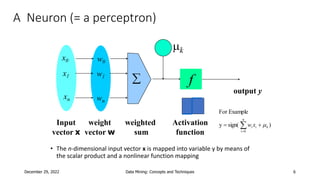
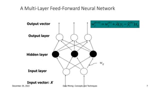
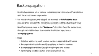
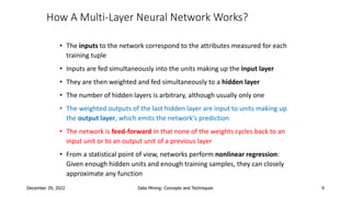
1
Data Mining:
Concepts and Techniques
(3rd ed.)
— Chapter 9 —
Classification: Advanced Methods
Jiawei Han, Micheline Kamber, and Jian Pei
University of Illinois at Urbana-Champaign &
Simon Fraser University
©2011 Han, Kamber & Pei. All rights reserved.
2
Chapter 9. Classification: Advanced Methods
• Classification by Backpropagation
3
Classification by Backpropagation
• Backpropagation: A neural network learning algorithm
• Started by psychologists and neurobiologists to develop and
test computational analogues of neurons
• A neural network: A set of connected input/output units where
each connection has a weight associated with it
• During the learning phase, the network learns by adjusting the
weights so as to be able to predict the correct class label of the
input tuples
• Also referred to as connectionist learning due to the
connections between units
4
Neural Network as a Classifier
• Weakness
• Long training time
• Require a number of parameters typically best determined empirically,
e.g., the network topology or “structure.”
• Poor interpretability: Difficult to interpret the symbolic meaning behind
the learned weights and of “hidden units” in the network
• Strength
• High tolerance to noisy data
• Ability to classify untrained patterns
• Well-suited for continuous-valued inputs and outputs
• Successful on an array of real-world data, e.g., hand-written letters
• Algorithms are inherently parallel
• Techniques have recently been developed for the extraction of rules from
trained neural networks
5
Neuron: A Hidden/Output Layer Unit
• An n-dimensional input vector x is mapped into variable y by means of the
scalar product and a nonlinear function mapping
• The inputs to unit are outputs from the previous layer. They are multiplied by
their corresponding weights to form a weighted sum, which is added to the bias
associated with unit. Then a nonlinear activation function is applied to it.
mk
f
weighted
sum
Input
vector x
output y
Activation
function
weight
vector w

w0
w1
wn
x0
x1
xn
)
sign(
y
Example
For
n
0
i
k
i
i x
w m

 

bias
December 29, 2022 Data Mining: Concepts and Techniques 6
A Neuron (= a perceptron)
• The n-dimensional input vector x is mapped into variable y by means of
the scalar product and a nonlinear function mapping
mk
-
f
weighted
sum
Input
vector x
output y
Activation
function
weight
vector w

w0
w1
wn
x0
x1
xn
)
sign(
y
Example
For
n
0
i
k
i
i x
w m

 

December 29, 2022 Data Mining: Concepts and Techniques 7
A Multi-Layer Feed-Forward Neural Network
Output layer
Input layer
Hidden layer
Output vector
Input vector: X
wij
ij
k
i
i
k
j
k
j x
y
y
w
w )
ˆ
( )
(
)
(
)
1
(





8
Backpropagation
• Iteratively process a set of training tuples & compare the network's prediction
with the actual known target value
• For each training tuple, the weights are modified to minimize the mean
squared error between the network's prediction and the actual target value
• Modifications are made in the “backwards” direction: from the output layer,
through each hidden layer down to the first hidden layer, hence
“backpropagation”
• Steps
• Initialize weights to small random numbers, associated with biases
• Propagate the inputs forward (by applying activation function)
• Backpropagate the error (by updating weights and biases)
• Terminating condition (when error is very small, etc.)
December 29, 2022 Data Mining: Concepts and Techniques 9
How A Multi-Layer Neural Network Works?
• The inputs to the network correspond to the attributes measured for each
training tuple
• Inputs are fed simultaneously into the units making up the input layer
• They are then weighted and fed simultaneously to a hidden layer
• The number of hidden layers is arbitrary, although usually only one
• The weighted outputs of the last hidden layer are input to units making up
the output layer, which emits the network's prediction
• The network is feed-forward in that none of the weights cycles back to an
input unit or to an output unit of a previous layer
• From a statistical point of view, networks perform nonlinear regression:
Given enough hidden units and enough training samples, they can closely
approximate any function
Sequence of Computations
1. Input and Output Processing at each hidden layer or output layer node:
j is the output layer or hidden layer node and i is a node in the previous layer connected to j
2. Error calculation at each unit j in the output layer:
where Tj is the Target Output while Oj is calculated output of the jth output unit
3. Error computation at a hidden layer unit j:
where wjk is the weight of the connection from unit j to an unit k in the next higher layer, and Errk is the error of unit k
4. Weight and bias updation:
December 29, 2022 Data Mining: Concepts and Techniques 10
 

i
j
i
ij
j O
w
I 
j
I
j
e
O 


1
1
)
)(
1
( j
j
j
j
j O
T
O
O
Err 


jk
k
k
j
j
j w
Err
O
O
Err 

 )
1
(
i
j
ij
ij O
Err
l
w
w )
(


j
j
j Err
l)
(



Example of Backpropagation Algorithm
Consider a 3-input, one output Neural Network with two hidden layer nodes:
1
2
3
5
4
6
x1
x2
x3
1,2,3 are input nodes, 4 and 5 hidden layer nodes, and 6 is output node
Dotted arrows indicate threshold values
w24
w14
w15
w25
w34
w35
w46
w56
𝜃4
𝜃5
𝜃6
Computed output of the network, O6
To be compared with T6 (the target
output or class label corresponding to
the given input vector (x1, x2, x3))
Feedforward Phase
Input Vector Weights
X1 = 1 w14 = 0.6
X2 = 0 w24 = 0.2 I4= 0.3 O4=0.57443 w46=-0.8
X3 = 1 w34 = -0.4
Bias 𝜃4 = 0.1
Bias 𝜃6 =-0.4 I6=-0.5594 O6=0.3637
Input Vector Weights
X1 = 1 w15 = 0.1
X2 = 0 w25 = 0.7 I5= 1.1 O5=0.75026 w56=0.4
X3 = 1 w35 = 0.3
Bias 𝜃5 = 0.7
 

i
j
i
ij
j O
w
I 
j
I
j
e
O 


1
1  

i
j
i
ij
j O
w
I 
j
I
j
e
O 


1
1
Error at Output Node
)
)(
1
( j
j
j
j
j O
T
O
O
Err 


Err6 = O6(1-O6)(T6 – O6)
Given T6 = 1 corresponding to the given input vector (x1, x2, x3)
Hence Err6 = 0.1473
Let l (learning rate) = 0.4
Backpropagation of Error to Hidden Layer
jk
k
k
j
j
j w
Err
O
O
Err 

 )
1
(
Err4 = O4(1-O4)Err6w46
Err4 = -0.02881
Err5 = O5(1-O5)Err6w56
Err5 = 0.01104
j=4
Error from all output nodes k are
backpropagated to the previous layer neuron j
k
As in our example there is only
one output node k, hence the
summation reduces to a single
term
j=5
Weight and bias updates
• Weight updates will happen at all the edges (connections) which are in the network: from input layer
to hidden layer, and hidden layer to output layer
If there is an edge between any two nodes i and j:
Let l (learning rate) = 0.4
w14 = w14 + l*Err4*O1 = 0.5908 (Note: O1 = x1 = 1, as there is no processing at input node)
w15 = 0.1044, w24 = 0.2 and w25 = 0.7 (no weight updation as O2 = x2 = 0), w34 = -0.41152, w35 = 0.30442,
w46 = -0.76615, w56 = 0.44421
• Bias updates will happen only at nodes where bias is present: hidden and output nodes
𝜃4 = 0.08848, 𝜃5 = 0.70442, 𝜃6 = -0.34108
i
j
ij
ij O
Err
l
w
w )
(


j
j
j Err
l)
(



i j
wij
Errj
Oi
You can play around with the learning rate
and see the variation….
l (learning rate) 0.4
Weights Biases
w14 0.611524 Theta4 0.111524
Node 6 0.147254 w15 0.1044 Theta5 0.704416
w34 -0.38848 Theta6 -0.34108
Node 4 0.028807 w35 0.304416
w46 -0.76615
Node 5 0.01104 w56 0.444205
Errors
Backpropagation of Error to Hidden Layer (general
case where there are more than one output nodes)
jk
k
k
j
j
j w
Err
O
O
Err 

 )
1
(
j
General Architecture of ANN
Error from all output nodes k are
backpropagated to the previous layer neuron j
.
.
.
.
.
.
k
As in our example there is only
one output node k, hence the
summation reduces to a single
term
Errj
Oj
wjk
Errk
More general case..If there was another hidden
layer
k
.
.
.
.
.
.
j
.
.
.
.
.
. .
.
.
.
.
.
.
.
Hidden
Layer H1
Hidden
Layer H2
By the same process the error
computation will happen in H1 after
H2
Error computation sequence:
First output layer (all nodes)
Then H2 (all nodes)
Then H1 (all nodes)
But no error computation in input
nodes (why?)
20
Defining a Network Topology
• Decide the network topology: Specify # of units in the input
layer, # of hidden layers (if > 1), # of units in each hidden layer,
and # of units in the output layer
• Normalize the input values for each attribute measured in the
training tuples to [0.0—1.0]
• One input unit per domain value, each initialized to 0
• Output, if for classification and more than two classes, one
output unit per class is used
• Once a network has been trained and its accuracy is
unacceptable, repeat the training process with a different
network topology or a different set of initial weights
21
Efficiency and Interpretability
• Efficiency of backpropagation: Each epoch (one iteration through the training
set) takes O(|D| * w), with |D| tuples and w weights, but # of epochs can be
exponential to n, the number of inputs, in worst case
• For easier comprehension: Rule extraction by network pruning
• Simplify the network structure by removing weighted links that have the
least effect on the trained network
• Then perform link, unit, or activation value clustering
• The set of input and activation values are studied to derive rules
describing the relationship between the input and hidden unit layers
• Sensitivity analysis: assess the impact that a given input variable has on a
network output. The knowledge gained from this analysis can be represented
in rules

10 Backpropagation Algorithm for Neural Networks (1).pptx

  • 1.
    1 Data Mining: Concepts andTechniques (3rd ed.) — Chapter 9 — Classification: Advanced Methods Jiawei Han, Micheline Kamber, and Jian Pei University of Illinois at Urbana-Champaign & Simon Fraser University ©2011 Han, Kamber & Pei. All rights reserved.
  • 2.
    2 Chapter 9. Classification:Advanced Methods • Classification by Backpropagation
  • 3.
    3 Classification by Backpropagation •Backpropagation: A neural network learning algorithm • Started by psychologists and neurobiologists to develop and test computational analogues of neurons • A neural network: A set of connected input/output units where each connection has a weight associated with it • During the learning phase, the network learns by adjusting the weights so as to be able to predict the correct class label of the input tuples • Also referred to as connectionist learning due to the connections between units
  • 4.
    4 Neural Network asa Classifier • Weakness • Long training time • Require a number of parameters typically best determined empirically, e.g., the network topology or “structure.” • Poor interpretability: Difficult to interpret the symbolic meaning behind the learned weights and of “hidden units” in the network • Strength • High tolerance to noisy data • Ability to classify untrained patterns • Well-suited for continuous-valued inputs and outputs • Successful on an array of real-world data, e.g., hand-written letters • Algorithms are inherently parallel • Techniques have recently been developed for the extraction of rules from trained neural networks
  • 5.
    5 Neuron: A Hidden/OutputLayer Unit • An n-dimensional input vector x is mapped into variable y by means of the scalar product and a nonlinear function mapping • The inputs to unit are outputs from the previous layer. They are multiplied by their corresponding weights to form a weighted sum, which is added to the bias associated with unit. Then a nonlinear activation function is applied to it. mk f weighted sum Input vector x output y Activation function weight vector w  w0 w1 wn x0 x1 xn ) sign( y Example For n 0 i k i i x w m     bias
  • 6.
    December 29, 2022Data Mining: Concepts and Techniques 6 A Neuron (= a perceptron) • The n-dimensional input vector x is mapped into variable y by means of the scalar product and a nonlinear function mapping mk - f weighted sum Input vector x output y Activation function weight vector w  w0 w1 wn x0 x1 xn ) sign( y Example For n 0 i k i i x w m    
  • 7.
    December 29, 2022Data Mining: Concepts and Techniques 7 A Multi-Layer Feed-Forward Neural Network Output layer Input layer Hidden layer Output vector Input vector: X wij ij k i i k j k j x y y w w ) ˆ ( ) ( ) ( ) 1 (     
  • 8.
    8 Backpropagation • Iteratively processa set of training tuples & compare the network's prediction with the actual known target value • For each training tuple, the weights are modified to minimize the mean squared error between the network's prediction and the actual target value • Modifications are made in the “backwards” direction: from the output layer, through each hidden layer down to the first hidden layer, hence “backpropagation” • Steps • Initialize weights to small random numbers, associated with biases • Propagate the inputs forward (by applying activation function) • Backpropagate the error (by updating weights and biases) • Terminating condition (when error is very small, etc.)
  • 9.
    December 29, 2022Data Mining: Concepts and Techniques 9 How A Multi-Layer Neural Network Works? • The inputs to the network correspond to the attributes measured for each training tuple • Inputs are fed simultaneously into the units making up the input layer • They are then weighted and fed simultaneously to a hidden layer • The number of hidden layers is arbitrary, although usually only one • The weighted outputs of the last hidden layer are input to units making up the output layer, which emits the network's prediction • The network is feed-forward in that none of the weights cycles back to an input unit or to an output unit of a previous layer • From a statistical point of view, networks perform nonlinear regression: Given enough hidden units and enough training samples, they can closely approximate any function
  • 10.
    Sequence of Computations 1.Input and Output Processing at each hidden layer or output layer node: j is the output layer or hidden layer node and i is a node in the previous layer connected to j 2. Error calculation at each unit j in the output layer: where Tj is the Target Output while Oj is calculated output of the jth output unit 3. Error computation at a hidden layer unit j: where wjk is the weight of the connection from unit j to an unit k in the next higher layer, and Errk is the error of unit k 4. Weight and bias updation: December 29, 2022 Data Mining: Concepts and Techniques 10    i j i ij j O w I  j I j e O    1 1 ) )( 1 ( j j j j j O T O O Err    jk k k j j j w Err O O Err    ) 1 ( i j ij ij O Err l w w ) (   j j j Err l) (   
  • 11.
  • 12.
    Example of BackpropagationAlgorithm Consider a 3-input, one output Neural Network with two hidden layer nodes: 1 2 3 5 4 6 x1 x2 x3 1,2,3 are input nodes, 4 and 5 hidden layer nodes, and 6 is output node Dotted arrows indicate threshold values w24 w14 w15 w25 w34 w35 w46 w56 𝜃4 𝜃5 𝜃6 Computed output of the network, O6 To be compared with T6 (the target output or class label corresponding to the given input vector (x1, x2, x3))
  • 13.
    Feedforward Phase Input VectorWeights X1 = 1 w14 = 0.6 X2 = 0 w24 = 0.2 I4= 0.3 O4=0.57443 w46=-0.8 X3 = 1 w34 = -0.4 Bias 𝜃4 = 0.1 Bias 𝜃6 =-0.4 I6=-0.5594 O6=0.3637 Input Vector Weights X1 = 1 w15 = 0.1 X2 = 0 w25 = 0.7 I5= 1.1 O5=0.75026 w56=0.4 X3 = 1 w35 = 0.3 Bias 𝜃5 = 0.7    i j i ij j O w I  j I j e O    1 1    i j i ij j O w I  j I j e O    1 1
  • 14.
    Error at OutputNode ) )( 1 ( j j j j j O T O O Err    Err6 = O6(1-O6)(T6 – O6) Given T6 = 1 corresponding to the given input vector (x1, x2, x3) Hence Err6 = 0.1473 Let l (learning rate) = 0.4
  • 15.
    Backpropagation of Errorto Hidden Layer jk k k j j j w Err O O Err    ) 1 ( Err4 = O4(1-O4)Err6w46 Err4 = -0.02881 Err5 = O5(1-O5)Err6w56 Err5 = 0.01104 j=4 Error from all output nodes k are backpropagated to the previous layer neuron j k As in our example there is only one output node k, hence the summation reduces to a single term j=5
  • 16.
    Weight and biasupdates • Weight updates will happen at all the edges (connections) which are in the network: from input layer to hidden layer, and hidden layer to output layer If there is an edge between any two nodes i and j: Let l (learning rate) = 0.4 w14 = w14 + l*Err4*O1 = 0.5908 (Note: O1 = x1 = 1, as there is no processing at input node) w15 = 0.1044, w24 = 0.2 and w25 = 0.7 (no weight updation as O2 = x2 = 0), w34 = -0.41152, w35 = 0.30442, w46 = -0.76615, w56 = 0.44421 • Bias updates will happen only at nodes where bias is present: hidden and output nodes 𝜃4 = 0.08848, 𝜃5 = 0.70442, 𝜃6 = -0.34108 i j ij ij O Err l w w ) (   j j j Err l) (    i j wij Errj Oi
  • 17.
    You can playaround with the learning rate and see the variation…. l (learning rate) 0.4 Weights Biases w14 0.611524 Theta4 0.111524 Node 6 0.147254 w15 0.1044 Theta5 0.704416 w34 -0.38848 Theta6 -0.34108 Node 4 0.028807 w35 0.304416 w46 -0.76615 Node 5 0.01104 w56 0.444205 Errors
  • 18.
    Backpropagation of Errorto Hidden Layer (general case where there are more than one output nodes) jk k k j j j w Err O O Err    ) 1 ( j General Architecture of ANN Error from all output nodes k are backpropagated to the previous layer neuron j . . . . . . k As in our example there is only one output node k, hence the summation reduces to a single term Errj Oj wjk Errk
  • 19.
    More general case..Ifthere was another hidden layer k . . . . . . j . . . . . . . . . . . . . . Hidden Layer H1 Hidden Layer H2 By the same process the error computation will happen in H1 after H2 Error computation sequence: First output layer (all nodes) Then H2 (all nodes) Then H1 (all nodes) But no error computation in input nodes (why?)
  • 20.
    20 Defining a NetworkTopology • Decide the network topology: Specify # of units in the input layer, # of hidden layers (if > 1), # of units in each hidden layer, and # of units in the output layer • Normalize the input values for each attribute measured in the training tuples to [0.0—1.0] • One input unit per domain value, each initialized to 0 • Output, if for classification and more than two classes, one output unit per class is used • Once a network has been trained and its accuracy is unacceptable, repeat the training process with a different network topology or a different set of initial weights
  • 21.
    21 Efficiency and Interpretability •Efficiency of backpropagation: Each epoch (one iteration through the training set) takes O(|D| * w), with |D| tuples and w weights, but # of epochs can be exponential to n, the number of inputs, in worst case • For easier comprehension: Rule extraction by network pruning • Simplify the network structure by removing weighted links that have the least effect on the trained network • Then perform link, unit, or activation value clustering • The set of input and activation values are studied to derive rules describing the relationship between the input and hidden unit layers • Sensitivity analysis: assess the impact that a given input variable has on a network output. The knowledge gained from this analysis can be represented in rules