Download as PDF, PPTX
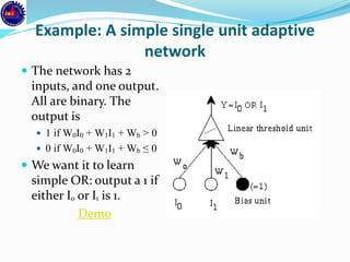
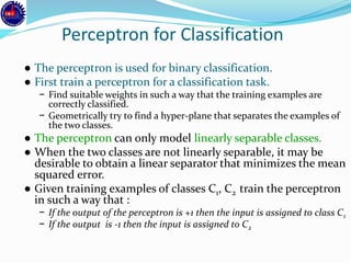
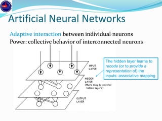
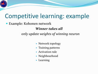
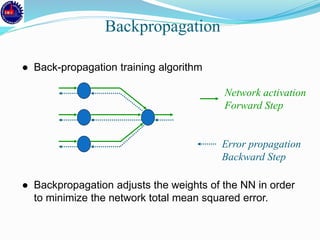
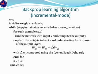
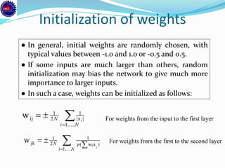
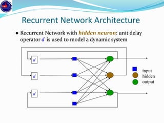
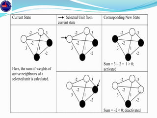
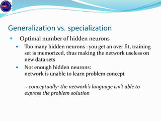
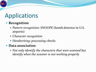
![Synapse concept
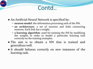
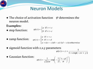
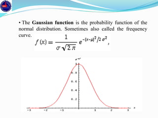
The synapse resistance to the incoming signal can be
changed during a "learning" process [1949]
Hebb’s Rule:
If an input of a neuron is repeatedly and persistently
causing the neuron to fire, a metabolic change
happens in the synapse of that particular input to
reduce its resistance](https://image.slidesharecdn.com/annppt-171207211618/85/Artificial-Neural-Network-7-320.jpg)
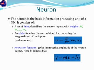
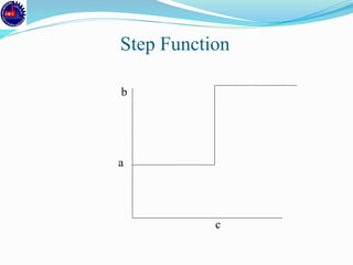
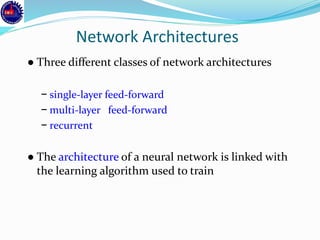
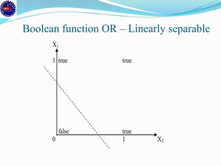
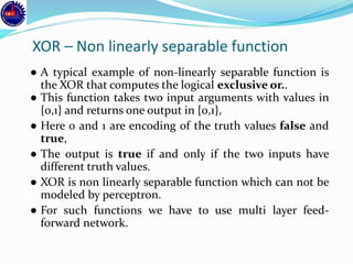
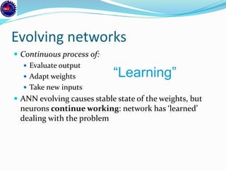
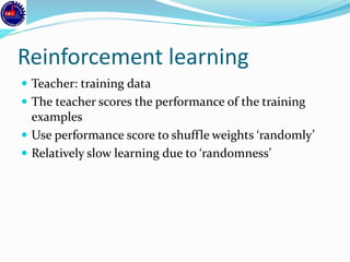
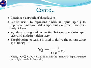
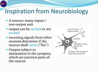
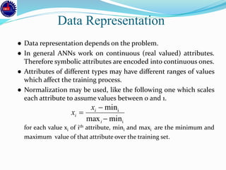
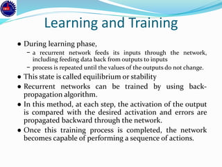
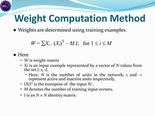
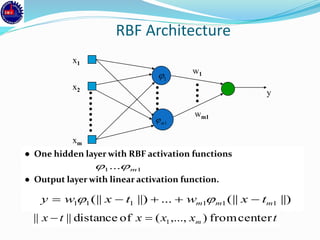
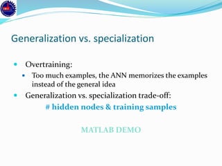
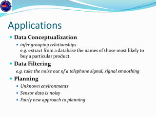
![Stopping criterions
● Total mean squared error change:
− Back-prop is considered to have converged when the absolute
rate of change in the average squared error per epoch is
sufficiently small (in the range [0.1, 0.01]).
● Generalization based criterion:
− After each epoch, the NN is tested for generalization.
− If the generalization performance is adequate then stop.
− If this stopping criterion is used then the part of the training set
used for testing the network generalization will not used for
updating the weights.](https://image.slidesharecdn.com/annppt-171207211618/85/Artificial-Neural-Network-47-320.jpg)

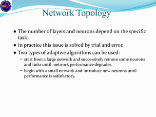
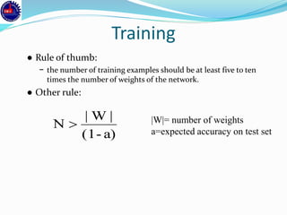
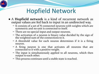
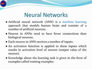
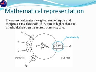
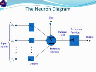
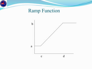
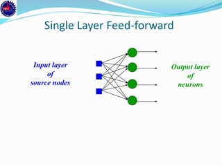
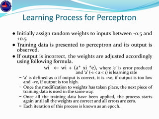
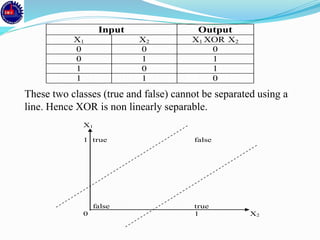
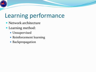
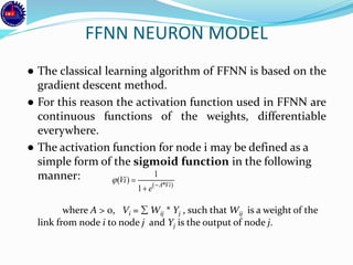
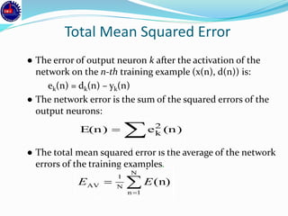
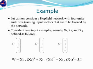
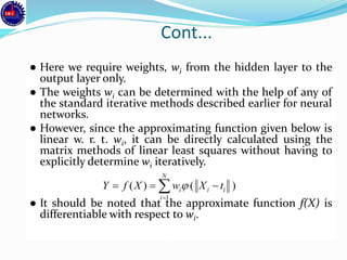
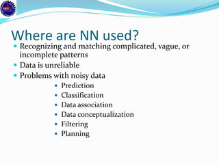
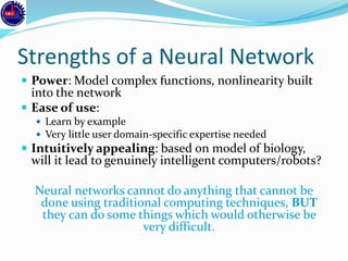
![1 2
1
1
–2
3
X=[011]
1 2
1
1
–2
3
X=[110]
1 2
1
1
–2
3
X=[000]
Stable Networks](https://image.slidesharecdn.com/annppt-171207211618/85/Artificial-Neural-Network-61-320.jpg)
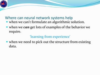
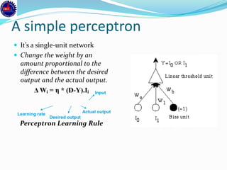
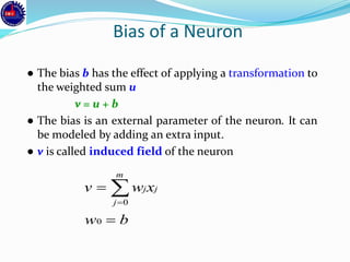
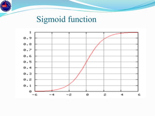
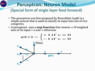
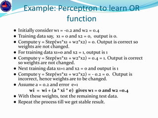
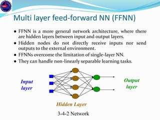
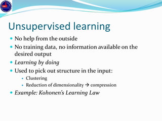
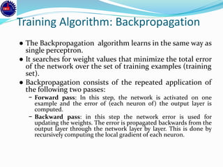
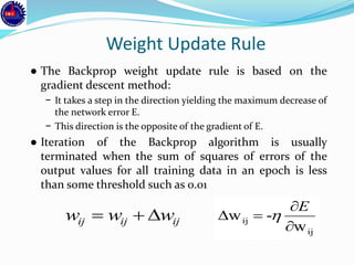
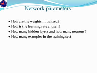
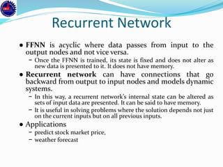
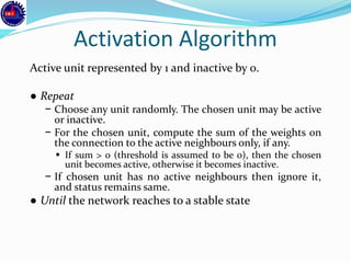
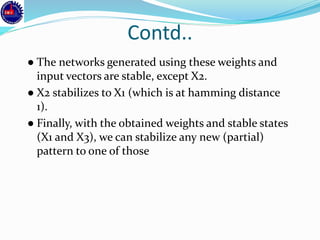
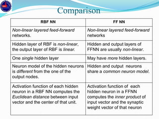
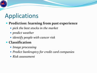
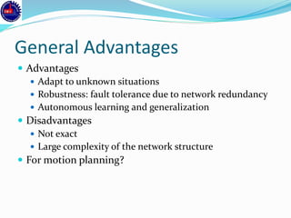
![3 –1 –3 3 3 0 0 0 0 –1 –3 3
W = –1 3 1 –1 . – 0 3 0 0 = –1 0 1 –1
–3 1 3 –3 0 0 3 0 –3 1 0 –3
3 –1 –3 3 0 0 0 3 3 –1 –3 0
X1 = [1 –1 –1 1]
1 -1 2
3 1
-3 -1
3 -3 4
X3 = [-1 1 1 -1]
1 -1 2
3 1
-3 -1
3 -3 4
Stable positions of the network](https://image.slidesharecdn.com/annppt-171207211618/85/Artificial-Neural-Network-64-320.jpg)


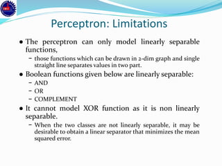
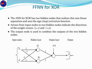
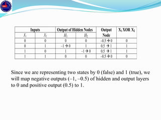
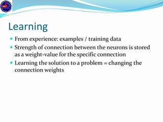
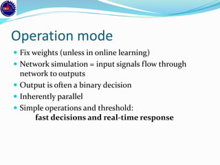
An artificial neural network (ANN) is a machine learning approach that models the human brain. It consists of artificial neurons that are connected in a network. Each neuron receives inputs and applies an activation function to produce an output. ANNs can learn from examples through a process of adjusting the weights between neurons. Backpropagation is a common learning algorithm that propagates errors backward from the output to adjust weights and minimize errors. While single-layer perceptrons can only model linearly separable problems, multi-layer feedforward neural networks can handle non-linear problems using hidden layers that allow the network to learn complex patterns from data.


![5G Explained! A High Level Overview [Introduction]](https://cdn.slidesharecdn.com/ss_thumbnails/5gexplainedahighleveloverview-260119165306-cc137a3e-thumbnail.jpg?width=640&height=640&fit=bounds)


