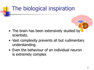
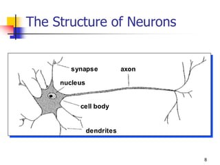
This document provides an overview of artificial neural networks. It discusses the biological inspiration from the brain and properties of artificial neural networks. Perceptrons and their limitations are described. Gradient descent and backpropagation algorithms for training multi-layer networks are introduced. Activation functions and network architectures are also summarized.


![21
Learning algorithm
Epoch : Presentation of the entire training set to the neural
network.
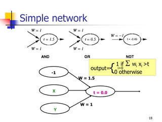
In the case of the AND function an epoch consists
of four sets of inputs being presented to the
network (i.e. [0,0], [0,1], [1,0], [1,1])
Error: The error value is the amount by which the value
output by the network differs from the target
value. For example, if we required the network to
output 0 and it output a 1, then Error = -1](https://image.slidesharecdn.com/ann-ics320part4-220419083124/85/ann-ics320Part4-ppt-21-320.jpg)
![22
Learning algorithm
Target Value, T : When we are training a network we
not only present it with the input but also with a
value that we require the network to produce. For
example, if we present the network with [1,1] for
the AND function the training value will be 1
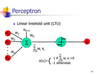
Output , O : The output value from the neuron
Ij : Inputs being presented to the neuron
Wj : Weight from input neuron (Ij) to the output neuron
LR : The learning rate. This dictates how quickly the
network converges. It is set by a matter of
experimentation. It is typically 0.1](https://image.slidesharecdn.com/ann-ics320part4-220419083124/85/ann-ics320Part4-ppt-22-320.jpg)


![35
Gradient Descent Learning
Rule
Consider linear unit without threshold and
continuous output o (not just –1,1)
o=w0 + w1 x1 + … + wn xn
Train the wi’s such that they minimize the
squared error
E[w1,…,wn] = ½ dD (td-od)2
where D is the set of training examples](https://image.slidesharecdn.com/ann-ics320part4-220419083124/85/ann-ics320Part4-ppt-35-320.jpg)
![36
Gradient Descent
D={<(1,1),1>,<(-1,-1),1>,
<(1,-1),-1>,<(-1,1),-1>}
Gradient:
E[w]=[E/w0,… E/wn]
(w1,w2)
(w1+w1,w2 +w2)
w=- E[w]
wi=- E/wi
=/wi 1/2d(td-od)2
= /wi 1/2d(td-i wi xi)2
= d(td- od)(-xi)](https://image.slidesharecdn.com/ann-ics320part4-220419083124/85/ann-ics320Part4-ppt-36-320.jpg)

![38
Incremental Stochastic
Gradient Descent
Batch mode : gradient descent
w=w - ED[w] over the entire data D
ED[w]=1/2d(td-od)2
Incremental mode: gradient descent
w=w - Ed[w] over individual training examples d
Ed[w]=1/2 (td-od)2
Incremental Gradient Descent can approximate Batch
Gradient Descent arbitrarily closely if is small
enough](https://image.slidesharecdn.com/ann-ics320part4-220419083124/85/ann-ics320Part4-ppt-38-320.jpg)


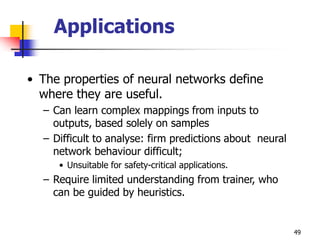
![48
Expressive Capabilities of
ANN
Boolean functions
Every boolean function can be represented by
network with single hidden layer
But might require exponential (in number of inputs)
hidden units
Continuous functions
Every bounded continuous function can be
approximated with arbitrarily small error, by network
with one hidden layer [Cybenko 1989, Hornik 1989]
Any function can be approximated to arbitrary
accuracy by a network with two hidden layers
[Cybenko 1988]](https://image.slidesharecdn.com/ann-ics320part4-220419083124/85/ann-ics320Part4-ppt-48-320.jpg)