The document covers the basics of arrays and matrices in MATLAB, explaining their structures, how to create and manipulate them, and the functions associated with them. It includes detailed examples of creating vectors and matrices, addressing elements, and performing mathematical operations such as addition, multiplication, and division. Moreover, it discusses built-in functions for generating matrices like zeros, ones, and random numbers, as well as approaches for appending and manipulating data in arrays.

1. LECTURE02
ARRAYS AND MATRICES
Shameer A Koya
1

2. An array is MATLAB's basic data
structure
• Can have any number of dimensions. Most common are
• vector - one dimension (a single row or column)
• matrix - two or more dimensions
• Scalar - matrices with only one row and one column.
• Arrays can have numbers or letters
2

3. Creating Matrices
• In MATLAB, a vector is created by assigning the elements of
the vector to a variable.
• This can be done in several ways depending on the source of
the information.
• —Enter an explicit list of elements
• —Load matrices from external data files
• —Using built-in functions
• —Using own functions in M-files
A matrix can be created in MATLAB by typing the elements
(numbers) inside square brackets [ ]
>> matrix = [1 2 3 ; 4 5 6 ; 7 8 9]
3

4. Examples
• >> A = [2 -3 5; -1 4 5]
A =
2 -3 5
-1 4 5
>> x = [1 4 7]
x =
1 4 7
>> x = [1; 4; 7]
x =
1
4
7
4
Note MATLAB displays row vector horizontally
Note MATLAB displays column vector vertically
Optional commas may be used between
the elements
Type the semicolon (or press Enter) to move to
the next row

5. >> cd=6; e=3; h=4;
>> Mat=[e cd*h cos(pi/3);h^2 sqrt(h*h/cd) 14]
Mat =
3.0000 24.0000 0.5000
16.0000 1.6330 14.0000
What if number of columns different?
>> B= [ 1:4; linspace(1,4,5) ]
??? Error using ==> vertcat
CAT arguments dimensions are not consistent.
5
Four columns Five columns

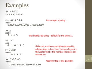
6. Create vector with specified constant
spacing between elements
The colon operator can be used to create a vector with constant
spacing
x = m:q:n
• m is first number
• n is last number
• q is difference between consecutive numbers
>>x=[1:2:10]
x =
1 3 5 7 9
If omit q, spacing is one
y = m:n
>> y=1:5
y =
1 2 3 4 5
6

7. Examples
>> x = 1:2:13
x = 1 3 5 7 9 11 13
>> >> 0.2:0.5:2.4
ans =
0.2000 0.7000 1.2000 1.7000 2.2000
>> 2:5
ans =
2 3 4 5
>> -2:3
ans =
-2 -1 0 1 2 3
>> -3:3:10
ans =
-3 0 3 6 9
>> 1.5:-0.5:-0.5
ans =
1.5000 1.0000 0.5000 0 -0.5000
7
Non-integer spacing
No middle step value - default for the step is 1.
negative step is also possible
If the last numbers cannot be obtained by
adding steps to first, then the last element in
the vector will be the number that does not
exceed last

8. Create vector with specified number of
terms b/w first and last
v = linspace( xi, xf, n )
• xi is first number
• xf is last number
• n is number of terms (= 100 if omitted)
>>f= linspace(0, 10, 5)
f =
0 2.5000 5.0000 7.5000 10.0000 5 elements, from 0 to 10
>>g= linspace(0, 10)
g =
Columns 1 through 10
0 0.1010 0.2020 0.3030 0.4040 ............................................
......................Columns 91 through 100
9.0909 9.1919 9.2929 9.3939 9.4949 9.5960 9.6970 9.7980
9.8990 10.0000
8

9. >> va = linspace( 0, 8, 6 )
va = 0 1.6000 3.2000 4.8000 6.4000 8.0000
>> va = linspace( 30, 10, 11 )
va=30 28 26 24 22 20 18 16 14 12 10
m:q:n lets you directly specify
spacing. linspace() lets you
directly specify number of terms
9
Six elements
Decreasing elements
T I P

10. Built-in Functions to Generate Matrices
zeros(r,c) - makes matrix of r rows and c
columns, all with zeros
ones(r,c) - makes matrix of r rows and c
columns, all with ones
rand(r,c) - makes matrix of r rows and c
columns, with random numbers
eye(n) - makes square matrix of n rows and
columns. Main diagonal (upper left to lower
right) has ones, all other elements are zero
magic(n) - makes a special square matrix of n
rows and c columns, called Durer’s matrix
10

11. Examples
>> a=zeros(3,4)
a = 0 0 0 0
0 0 0 0
0 0 0 0
>> b=ones(4,3)
b = 1 1 1
1 1 1
1 1 1
1 1 1
>> c = rand(2,3)
c =
0.8147 0.1270 0.6324
0.9058 0.9134 0.0975
11
>> d=eye(4)
d = 1 0 0 0
0 1 0 0
0 0 1 0
0 0 0 1
>> e=magic(4)
e = 16 2 3 13
5 11 10 8
9 7 6 12
4 14 15 1

12. To make a matrix filled with a particular
number, multiply ones(m,n) by that
number
>> z=100*ones(3,4)
z =
100 100 100 100
100 100 100 100
100 100 100 100 12
T I P

13. Functions to Handle Matrices and Arrays
• length( ) - number of elements in a array. number of columns in a
matrix
• >>length(y)
• ans =
• 3
• >>length(x)
• ans =
• 3
•
• sum( ) – Sum of elements in a array. Sum of elements in a column of
a matrix.
• >>sum(x)
• ans =
• 6
• >>sum(y)
• ans =
• 5 7 9
13
x = [1 2 3];
y= [1 2 3; 4 5 6];

14. Functions to Handle Matrices and Arrays
‘ – Transpose of a matrix. Convert a row vector to column vector
>>y'
ans =
1 4
2 5
3 6
>> x'
ans =
1
2
3
diag( ) – diagonal elements of matrix. crate a matrix with elements of a vector,if the
argument is a vector)
>>diag(y)
ans =
1
5
>>diag(x)
ans =
1 0 0
0 2 0
0 0 3
14
x = [1 2 3];
y= [1 2 3; 4 5 6];

15. Functions to Handle Matrices and Arrays
• size( ) – size (dimensions) of matrix
>>size(y)
ans =
2 3 (2 rows, 3 columns)
•
det( ) – determinant of a matrix. (matrix must be square to get
determinant)
• >> z= [1 2 3; 4 5 6; 7 8 0];
• >> det (z)
• ans =
• 27
•
• inv( ) – inverse of a square matrix
• >> inv(z)
• ans =
• -1.7778 0.8889 -0.1111
• 1.5556 -0.7778 0.2222
• -0.1111 0.2222 -0.1111
15
x = [1 2 3];
y= [1 2 3; 4 5 6];

16. Subscripts and Extracting a Sub-Matrix
Can access (read from or write to) elements in
array (vector or matrix) individually or in groups
• Useful for changing subset of elements
• Useful for making new variable from subset of elements
• Address (index) of element is its position in the array
• x(n) – nth element in the vector
• x(i, j)- element in ith row, jth column
16

17. Examples
>> A=[35 46 78 23 5 14 81 3 55]
A = 35 46 78 23 5 14 81 3 5
>> A(4)
ans = 23
>> A(6)=27
A = 35 46 78 23 5 27 81 3 5
>> A(2)+A(8)
ans = 49
>> A(5)^A(8)+sqrt(A(7))
ans = 134
17

18. >> MAT=[3 11 6 5; 4 7 10 2; 13 9 0 8]
MAT = 3 11 6 5
4 7 10 2
13 9 0 8
>> MAT(3,1)
ans = 13
>> MAT(3,1)=20
MAT = 3 11 6 5
4 7 10 2
20 9 0 8
>> MAT(2,4)-MAT(1,2)
ans = -9 18
Element in
row 3 and
column 1
Assign new value to element in row 3 and column 1
Only this
element
changed
Column 1
Row 3

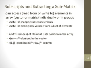
19. Using a Colon : in Addressing Arrays
The colon : lets you address a range
of elements
• Vector (row or column)
• x(:) - all elements
• x(m:n) - elements m through n
• Matrix
• A(:,n) - all rows of column n
• A(m,:) - all columns of row m
• A(:,m:n) - all rows of columns
m through n
• A(m:n,:) - all columns of rows
m through n
• A(m:n,p:q) - columns p
through q of rows
m through n
19
• >> A(3,:) % extract the 3rd row
• ans =
7 8 9
• >> A(:,2) % extract the 2nd
column
• ans =
2
5
8
• >> A([1,3],1:2) % extract 1st and
2nd elements of 1st and 3rd rows
• ans =
1 2
7 8

20. Adding And Deleting Elements
• Indexing can be used to add and delete
elements from a matrix.
• >> A(5,2) = 5 % assign 5 to the position (5,2);
the uninitialized elements become zeros
• >> A(4,:) = [2, 1, 2]; % assign vector [2, 1, 2] to the
4th row of A
• >> A(5,[1,3]) = [4, 4]; % assign: A(5,1) = 4 and
A(5,3) = 4
• A(4,:) = [ ] - will delete 4th row
• A(:, 3) = [ ] – will delete 3rd column
• A(1,2) = [ ] – error
• Can’t delete single element in a row or column.
20
A =
1 2 3
4 5 8
7 8 9
0 0 0
0 5 0
A(2:2:6) = [ ]
ans = 1 7 5 3 6 9
……………. How?

21. More Examples
v = 4 7 10 13 16 19 22 25 28 31 34
>> u=v([3, 5, 7:10])
u = 10 16 22 25 28 31
>> u=v([3 5 7:10])
u = 10 16 22 25 28 31
DF = 1 2 3 4
>> DF(5:7)=10:5:20
DF = 1 2 3 4 10 15 20
>> DF(10)=50
DF = 1 2 3 4 10 15 20 0 0 50
>> A=[10:-1:4; ones(1,7); 2:2:14; zeros(1,7)]
A = 10 9 8 7 6 5 4
1 1 1 1 1 1 1
2 4 6 8 10 12 14
0 0 0 0 0 0 0
>> B=A([1 3],[1 3 5:7])
B = 10 8 6 5 4
2 6 10 12 14
21

22. Appending vectors and matrices
• Can only append row vectors to row vectors and column vectors
to column vectors
• If r1 and r2 are any row vectors,
r3 = [r1 r2] is a row vector whose left part is r1 and right part
is r2
• If c1 and c2 are any column vectors,
c3 = [c1; c2] is a column vector whose top part is c1 and
bottom part is c2
• If appending one matrix to right side of other matrix, both must
have same number of rows
• If appending one matrix to bottom of other matrix, both must
have same number of columns
22

23. Examples
r = [r1,r2]
r =
1 2 3 4 5 6 7 8
c = [c1; c2]
>> Z=[A B]
Z = 1 2 3 7 8
4 5 6 9 10
>> Z=[A; C]
Z = 1 2 3
4 5 6
1 0 0
0 1 0
0 0 1
>> Z=[A; B]
??? Error using ==> vertcat
CAT arguments dimensions are not
consistent.
23
r1 = [1 2 3 4 ]
r2 = [5 6 7 8 ]
c1 = [1; 2; 3; 4 ]
c2 = [5; 6; 7; 8 ]
A = 1 2 3
4 5 6
B = 7 8
9 10
C = 1 0 0
0 1 0
0 0 1
c =
1
2
3
4
5
6
7
8

24. Operations on Matrices
• Previously dealt with scalars (single numbers). Will now
work with arrays, which in general have more than one
number
24

25. Addition and Subtraction
When adding/ subtracting two arrays A and B, MATLAB
adds/subtracts the corresponding elements (element wise
addition/subtraction)
When add/subtract a scalar to an array, MATLAB adds /
subtracts the scalar to every element of the array
25

26. Matrix Multiplication
There are two ways of multiplying matrices – matrix
multiplication and elementwise multiplication
MATRIX MULTIPLICATION
• MATLAB denotes this with asterisk (*)
• Number of columns in left matrix must be same as number of rows
in right matrix
26

27. Matrix multiplication on two vectors
• They must both be the
same size
• One must be a row vector
and the other a column
vector
• If the row vector is on the
left, the product is a scalar
• If the row vector is on the
right, the product is a
square matrix whose side is
the same size as the vectors
27
>> h = [ 2 4 6 ]
h =
2 4 6
>> v = [ -1 0 1 ]'
v =
-1
0
1
>> h * v
ans =
4
>> v * h
ans =
-2 -4 -6
0 0 0
2 4 6

28. Array Division
Left division, :
Left division is one of MATLAB's two kinds of array
division
• Used to solve the matrix equation AX=B
• A is a square matrix, X, B are column vectors
• Solution is X = A-1B
In MATLAB, solve by using left division operator (), i.e.,
>> X = A B
When solving set of linear equations, use left division,
not inverse, i.e., use X=AB not X=inv(A)*B
Left division is
• 2-3 times faster
• Often produces smaller error than inv()
• Sometimes inv()can produce erroneous results
28

29. Right division, /:
Right division is the other kind of MATLAB's array
division
• Used to solve the matrix equation XC=D
• C is a square matrix, X, D are row vectors
• Solution is X = D·C-1
In MATLAB, solve by using right division operator
(/), i.e.,
>> X = D / C
29

30. Element-by-Element Operations
• Addition and subtraction of arrays is always elementwise
• Multiplication, division, exponentiation of arrays can be
elementwise
• Both arrays must be same dimension
30

31. Example
ELEMENTWISE MULTIPLICATION
>> A = [1 2; 3 4];
>> B = [0 1/2; 1 -1/2];
>> C = [1 0]’;
>> D = A .* B
D =
0 1
3 -2
>> A .* C
??? Error using ==> times
Matrix dimensions must agree.
31

32. Built-in Functions for Analyzing Arrays
• mean(v) – mean (average)
• max(v) – maximum value, optionally with index of maximum
• min(v) – minimum value, optionally with index of minimum
• sum(v) – sum
• sort(v) – elements sorted into ascending order
• median(v) – median
• std(v) – standard deviation
• dot(v,w) – dot (inner product); v, w both vectors of same
size but any dimension
• cross(v,w) – cross product; v, w must both have three
elements but any dimension
32

33. 33
Multi-dimensional Array
•Arrays can have more than two dimensions
•A= [ 1 2; 3 4]
•You can add the 3rd dimension by
•A(:,:,2) = [ 5 6; 7 8]