Computer Network Routing Techniques

1. Routing Techniques
UNIT II

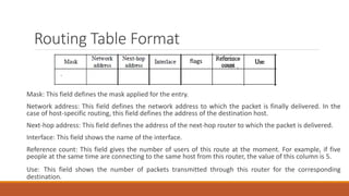
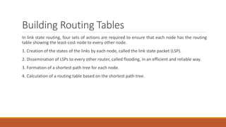
2. Static Routing
A static routing table contains information entered manually. The administrator enters the route
for each destination into the table. When a table is created, it cannot update automatically
when there is a change in the Internet.
The table must be manually altered by the administrator.

3. Dynamic Routing Table
A dynamic routing table is updated periodically by using one of the dynamic routing protocols
such as RIP, OSPF, or BGP.
Whenever there is a change in the Internet, such as a shutdown of a router or breaking of a link,
the dynamic routing protocols update all the tables in the routers (and eventually in the host)
automatically.

4. Routing Table Format
Mask: This field defines the mask applied for the entry.
Network address: This field defines the network address to which the packet is finally delivered. In the
case of host-specific routing, this field defines the address of the destination host.
Next-hop address: This field defines the address of the next-hop router to which the packet is delivered.
Interface: This field shows the name of the interface.
Reference count: This field gives the number of users of this route at the moment. For example, if five
people at the same time are connecting to the same host from this router, the value of this column is 5.
Use: This field shows the number of packets transmitted through this router for the corresponding
destination.
flags

5. Flags. This field defines up to five flags. Flags are on/off switches that signify either presence or
absence. The five flags are U (up), G (gateway), H (host-specific), D (added by redirection), and M
(modified by redirection).
◦ U (up). The U flag indicates the router is up and running. If this flag is not present, it means that the router is
down. The packet cannot be forwarded and is discarded.
◦ G (gateway). The G flag means that the destination is in another network. The packet is delivered to the next-
hop router for delivery (indirect delivery). When this flag is missing, it means the destination is in this
network (direct delivery).
◦ H (host-specific). The H flag indicates that the entry in the network address field is a host-specific address.
When it is missing, it means that the address is only the network address of the destination.
◦ D (added by redirection). The D flag indicates that routing information for this destination has been added to
the host routing table by a redirection message from ICMP.
◦ M (modified by redirection). The M flag indicates that the routing information for this destination has been
modified by a redirection message from ICMP.

6. Distance Vector Routing
• In distance vector routing, the least-cost
route between any two nodes is the route
with minimum distance.
• In this protocol, as the name implies, each
node maintains a vector (table) of
minimum distances to every node.
• The table at each node also guides the
packets to the desired node by showing
the next stop in the route (next-hop
routing)

7. …
The whole idea of distance vector routing is
the sharing of information between
neighbours.
Although node A does not know about node
E, node C does. So if node C shares its
routing table with A, node A can also know
how to reach node E.
On the other hand, node C does not know
how to reach node D, but node A does. If
node A shares its routing table with node C,
node C also knows how to reach node D.
In other words, nodes A and C, as immediate
neighbours, can improve their routing tables
if they help each other.

8. Distance Vector vs Link State

9. Link State Routing Process
1. Each router learns about its own links (directly connected networks)
2. Find directly connected neighbours.
3. Builds a Link-State Packet (LSP) with the state of each directly connected link
4. Floods the LSP to all neighbours, who stores the received LSPs in a database
5. Each router uses the database to construct a complete map of the network topology
6. Computes the best path to each destination network

10. Advantages with Link-State Protocols
• Builds a topological map
◦ – Full knowledge of the network
• Fast convergence
◦ – Floods LSPs immediately
• Event-driven updates
◦ – LSP sent when there is a change, only contains information regarding the affected link
• Hierarchical design
◦ – Areas can be used to separate routing traffic

11. Disadvantages with Link-State Protocol
• Significant demands on memory and processing resources.
• Requires very strict network design.
• Requires a knowledgeable network administrator.
• Initial flooding can impede network performance.

12. Link-State Routing Features
Hello protocol
– Used to discover and maintain neighbour
adjacencies

13. Link State Knowledge

14. Building Routing Tables
In link state routing, four sets of actions are required to ensure that each node has the routing
table showing the least-cost node to every other node.
1. Creation of the states of the links by each node, called the link state packet (LSP).
2. Dissemination of LSPs to every other router, called flooding, in an efficient and reliable way.
3. Formation of a shortest path tree for each node.
4. Calculation of a routing table based on the shortest path tree.

15. Creation of Link State Packet (LSP)
A link state packet can carry a large amount of information. For the moment, however, we
assume that it carries a minimum amount of data:
1. The node identity,
2. The list of links,
3. A sequence number
4. Age
LSPs are generated on two occasions:
1. When there is a change in the topology of the domain
2. Updates On a periodic basis

16. Multicast Routing
In multicast communication, there is one source and a group of destinations. The relationship is
one-to-many. In this type of communication, the source address is a unicast address, but the
destination address is a group address, which defines one or more destinations. The group
address identifies the members of the group.
A multicast packet starts from the source S1 and goes to all destinations that belong to group
G1. In multicasting, when a router receives a packet, it may forward it through several of its
interfaces.
In multicasting, the router may forward the received packet through several of its interfaces.

18. Data Traffic
The main focus of congestion control and quality of service is data traffic. In congestion control
we try to avoid traffic congestion. In quality of service, we try to create an appropriate
environment for the traffic. So, before talking about congestion control and quality of service,
we discuss the data traffic itself.

19. Traffic Descriptor
Traffic descriptors are qualitative values that represent a data flow.
1. Average Data Rate
The average data rate is the number of bits sent during a period of time, divided by the number of
seconds in that period.
2. Peak Data Rate
The peak data rate defines the maximum data rate of the traffic. It is a very important measurement
because it indicates the peak bandwidth that the network needs for traffic to pass through without
changing its data flow.
3. Maximum Burst Size
The maximum burst size normally refers to the maximum length of time the traffic is generated at the
peak rate.
4. Effective Bandwidth
The effective bandwidth is the bandwidth that the network needs to allocate for the flow of traffic.

20. Traffic Profiles
1. Constant Bitrate
A constant-bit-rate (CBR), or a fixed-rate, traffic model has a data rate that does not change. In
this type of flow, the average data ratc and thc peak data rate are the same.
2. Variable Bitrate
In the variable-bit-rate (VBR) category, the rate of the data flow changes in time, withthe
changes smooth instead of sudden and sharp. In this type of flow, the average data rate and the
peak data rate are different. The maximum burst size is usually a small value.
3. Bursty
In the bursty data category, the data rate changes suddenly in a very short time. It may jump
from zero, for example, to 1 Mbps in a few microseconds and vice versa. It may also remain at
this value for a while. The average bit rate and the peak bit rate are very different values in this
type of flow. The maximum burst size is significant.

21. Congestion
Congestion in a network may occur if the load on the network-the number of packets sent to
the network-is greater than the capacity of the network-the number of packets a network can
handle.
Congestion in a network or internetwork occurs because routers and switches have queues-
buffers that hold the packets before and after processing.

22. CONGESTION CONTROL
Congestion control refers to techniques and mechanisms that can either prevent congestion,
before it happens, or remove congestion, after it has happened.
In general, we can divide congestion control mechanisms into two broad categories:
1. Open-loop congestion control (prevention)
2. Closed-loop congestion control (removal)

23. Open-Loop Congestion Control
1. Retransmission Policy: Retransmission is sometimes unavoidable. If the sender feels that a
sent packet is lost or corrupted, the packet needs to be retransmitted
2. Window Policy: The type of window at the sender may also affect congestion. The Selective
Repeat window is better than the Go-Back-N window for congestion control.
3. Acknowledgement Policy: The acknowledgment policy imposed by the receiver may also
affect congestion. If the receiver does not acknowledge every packet it receives, it may slow
down the sender and help prevent congestion.
4. Discarding Policy: A good discarding policy by the routers may prevent congestion and at the
same time may not harm the integrity of the transmission. For example, in audio transmission, if
the policy is to discard less sensitive packets when congestion is likely to happen
5. Admission Policy: An admission policy, which is a quality-of-service mechanism, can also
prevent congestion in virtual-circuit networks.

24. Closed Loop Congestion
1. Backpressure: The technique of backpressure refers to a congestion control mechanism in
which a congested node stops receiving data from the immediate upstream node or nodes. This
may cause the upstream node or nodes to become congested, and they, in turn, reject data from
their upstream nodes or nodes.
Backpressure is a node-to-node congestion control that starts with a node and propagates, in
the opposite direction of data flow, to the source. The backpressure technique can be applied
only to virtual circuit networks, in which each node knows the upstream node from which a flow
of data is corning.

25. …
2. Choke Packet: In choke-packet the warning of the congestion is directly sent by the router to
the source address to stop or to slow down the transmission. The intermediate nodes will not be
warned the congestion like in backpressure technique.

26. Implicit Signalling
In implicit signalling, there is no communication between the congested node or nodes and the
source. The source guesses that there is a congestion somewhere in the network from other
symptoms.
For example, when a source sends several packets and there is no acknowledgment for a while,
one assumption is that the network is congested. The delay in receiving an acknowledgment is
interpreted as congestion in the network; the source should slow down.

27. Explicit Signalling
Backward Signalling: A bit can be set in a packet moving in the direction opposite to the
congestion. This bit can warn the source that there is congestion and that it needs to slow down
to avoid the discarding of packets.
Forward Signalling: A bit can be set in a packet moving in the direction of the congestion. This
bit can warn the destination that there is congestion. The receiver in this case can use policies,
such as slowing down the acknowledgments, to alleviate the congestion.

28. Quality of Service
Flow Characteristics
Four types of characteristics are attributed to
the flow.
1. Reliability: Reliability is a characteristic that a
flow needs. Lack of reliability means losing a
packet or acknowledgment, which entails
retransmission.
2.Delay: Source-to-destination delay is another
flow characteristic. Again applications can
tolerate delay in different degrees.
3.Jitter: Jitter is the variation in delay for packets
belonging to the same flow.
4.Bandwidth: Different applications need
different bandwidths.

29. Techniques to improve QOS
Broadly there are four common techniques:
1. Scheduling
◦ FiFo Queuing
◦ Priority Queuing
2. Traffic Shaping:Traffic shaping is a mechanism to control the amount and the rate of the
traffic sent to the network.
◦ Leaky Bucket
◦ Token Bucket
3. Admission Control
4. Resource Reservation

30. Leaky Bucket
If a bucket has a small hole at the bottom, the water leaks
from the bucket at a constant rate as long as there is water
in the bucket. The rate at which the water leaks does not
depend on the rate at which the water is input to the
bucket unless the bucket is empty. The input rate can vary,
but the output rate remains constant. Similarly, in
networking, a technique called leaky bucket can smooth
out bursty traffic.
A leaky bucket algorithm shapes bursty traffic into fixed-rate traffic by averaging the data rate.
It may drop the packets if the bucket is full.

31. Leaky Bucket Implementation
Arrival Departure
The following is an algorithm for variable-length packets:
1. Initialize a counter to n at the tick of the clock.
2. If n is greater than the size of the packet, send the packet and decrement the counter by the
packet size. Repeat this step until n is smaller than the packet size.
3. Reset the counter and go to step 1.

32. Token Bucket
The leaky bucket is very restrictive. It does not credit an idle host.
For example, if a host is not sending for a while, its bucket becomes empty. Now if the host has
bursty data, the leaky bucket allows only an average rate.
The time when the host was idle is not taken into account. On the other hand, the token bucket
algorithm allows idle hosts to accumulate credit for the future in the form of tokens. For each
tick of the clock, the system sends n tokens to the bucket. The system removes one token for
every cell (or byte) of data sent.
For example, if n is 100 and the host is idle for 100 ticks, the bucket collects 10,000 tokens. Now
the host can consume all these tokens in one tick with 10,000 cells, or the host takes 1000 ticks
with 10 cells per tick.
The token bucket allows bursty traffic at a regulated maximum rate.

34. Resource Reservation
A flow of data needs resources such as a buffer, bandwidth, CPU time, and so on. The quality of
service is improved if these resources are reserved beforehand. We discuss in this section one QoS
model called Integrated Services, which depends heavily on resource reservation to improve the
quality of service.
Admission Control
Admission control refers to the mechanism used by a router, or a switch, to accept or reject a flow
based on predefined parameters called flow specifications. Before a router accepts a flow for
processing, it checks the flow specifications to see if its capacity (in terms of bandwidth, buffer size,
CPU speed, etc.) and its previous commitments to other flows can handle the new flow.

35. IPV4
IPv4 is an unreliable and connectionless datagram protocol-a best-effort delivery service. The
term best-effort means that IPv4 provides no error control or flow control (except for error
detection on the header). IPv4 assumes the unreliability of the underlying layers and does its
best to get a transmission through to its destination, but with no guarantees.

36. IPV4 Datagram
A datagram is a variable-length
packet consisting of two parts:
header and data.
The header is 20 to 60 bytes in
length and contains information
essential to routing and delivery.
It is customary in TCP/IP to show
the header in 4-byte sections.
A brief description of each field is
in order.

37. …
• VER: This 4-bit field defines the version of the IPv4 protocol. Currently the version is 4. However
• HLEN: This 4-bit field defines the total length of the datagram header in 4-byte words.
• Services
• Total Length: The total length field defines the total length of the datagram including the header.
• Identification: This field is used in fragmentation
• Flags: This field is used in fragmentation
• Fragmentation offset: This field is used in fragmentation
• Time to Live: A datagram has a limited lifetime in its travel through an internet. This field was originally designed
to hold a timestamp, which was decremented by each visited router. The datagram was discarded when the value
became zero.
• Protocol
• Checksum
• Source Address
•Destination Address