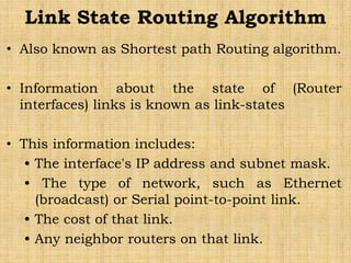
Downloaded 24 times


![The DV calculation is based on minimizing the cost to
each destination.
Dx(y) = Estimate of least cost from x to y
C(x,v) = Node x knows cost to each neighbor v
Dx = [Dx(y): y ∈ N ] = Node x maintains distance vector
Node x also maintains its neighbors' distance vectors
– For each neighbor v, x maintains Dv = [Dv(y): y ∈ N ]
• From time-to-time, each node sends its own distance
vector estimate to neighbors.
• When a node x receives new DV estimate from any
neighbor v, it saves v’s distance vector and it updates
its own DV using B-F equation:
Dx(y) = min { C(x,v) + Dv(y)} for each node y ∈ N](https://image.slidesharecdn.com/routingalgorithms-200106064529/85/Routing-algorithms-9-320.jpg)


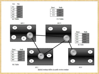


The document discusses routing algorithms, detailing both adaptive and non-adaptive types, their classifications, and specific algorithms such as distance vector and link state routing. Adaptive algorithms adjust routing decisions based on network conditions, while non-adaptive algorithms use pre-computed routes. The document also covers the workings of various routing algorithms, their advantages and disadvantages, and the role of speaker nodes in path vector routing.