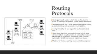
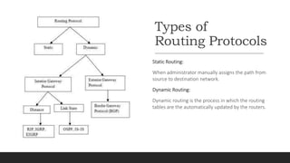
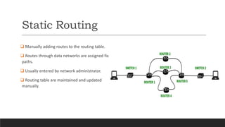
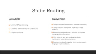
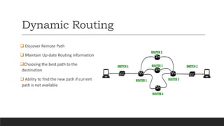
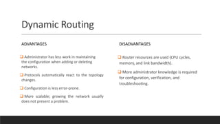
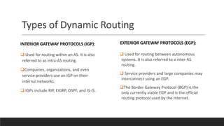
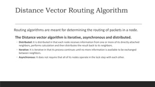
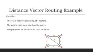
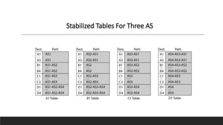
- Routing protocols are used by routers to communicate and determine the best paths between networks. They update routing tables but do not actually transmit data. - There are static and dynamic routing protocols. Static routing uses manually configured paths while dynamic routing automatically updates paths in response to network changes. - Common routing protocols include RIP, OSPF, BGP, which use different algorithms like distance vector or link state to calculate paths. Dijkstra's algorithm is an example used in link state routing to find shortest paths through a network.

1. Ehtisham Murtaza
19011556-030
Saad Ahmad
19011556-001
Mirza Umair
19011556-002
Group No:6
Routing Protocols

2. Routing
Protocols
 Routing protocols are the set of rules used by the the
routers to communicate with the source and the destination.
 Routing protocols don’t move the information from source
to destination they only updates the routing tables.
 Each protocol has its own algorithm to choose the best
path.
 Main Goals of Routing Protocols To fill the routing table
with current best, loop-free routes To notice when routes in
the table are no longer valid and remove them from the
routing table To add new routes or replace lost routes
The time for finding a working route is called convergence.

3. Types of
Routing Protocols
Static Routing:
When administrator manually assigns the path from
source to destination network.
Dynamic Routing:
Dynamic routing is the process in which the routing
tables are the automatically updated by the routers.

4. Static Routing
 Manually adding routes to the routing table.
 Routes through data networks are assigned fix
paths.
 Usually entered by network administrator.
 Routing table are maintained and updated
manually.

5. Static Routing
ADVANTAGES
 Minimal CPU processing
 Easier for administrator to understand
 Easy to configure
DISADVANTAGES
 Configuration and maintenance are time-consuming.
 Configuration is error-prone, especially in large
networks.
 Administrator intervention is required to maintain
changing route information.
 Does not scale well with growing networks;
maintenance becomes cumbersome.
 Requires complete knowledge of the entire network
for proper implementation.

6. Dynamic Routing
 Discover Remote Path
 Maintain Up-date Routing information
Choosing the best path to the
destination
 Ability to find the new path if current
path is not available

7. Dynamic Routing
ADVANTAGES
 Administrator has less work in maintaining
the configuration when adding or deleting
networks.
 Protocols automatically react to the topology
changes.
 Configuration is less error-prone.
 More scalable; growing the network usually
does not present a problem.
DISADVANTAGES
 Router resources are used (CPU cycles,
memory, and link bandwidth).
 More administrator knowledge is required
for configuration, verification, and
troubleshooting.

8. Autonomous
System
 As is the collection of the networks under the
common administration and sharing a common
routing strategy.
 AS divides the global networks into the smaller and
more meaningful networks.
 Each As has its own set of rules and policies.
 The AS number uniquely differ it from other AS in
the word.

9. Types of Dynamic Routing
INTERIOR GATEWAY PROTOCOLS (IGP): EXTERIOR GATEWAY PROTOCOLS (EGP):
 Used for routing between autonomous
systems. It is also referred to a inter-AS
routing.
 Service providers and large companies may
interconnect using an EGP.
The Border Gateway Protocol (BGP) is the
only currently viable EGP and is the official
routing protocol used by the Internet.
 Used for routing within an AS. It is also
referred to as intra-AS routing.
Companies, organizations, and even
service providers use an IGP on their
internal networks.
 IGPs include RIP, EIGRP, OSPF, and IS-IS.

10. Distance Vector Routing Algorithm
Routing algorithms are meant for determining the routing of packets in a node.
The Distance vector algorithm is iterative, asynchronous and distributed.
◦ Distributed: It is distributed in that each node receives information from one or more of its directly attached
neighbors, performs calculation and then distributes the result back to its neighbors.
◦ Iterative: It is iterative in that its process continues until no more information is available to be exchanged
between neighbors.
◦ Asynchronous: It does not require that all of its nodes operate in the lock step with each other.

11. The Distance vector algorithm is a dynamic algorithm.
It is mainly used in ARPANET, and RIP.
Each router maintains a distance table known as Vector.

12. Three Keys to understand the working
of Distance Vector Routing Algorithm
Knowledge about the whole network: Each router shares its knowledge through the
entire network. The Router sends its collected knowledge about the network to its
neighbors.
Routing only to neighbors: The router sends its knowledge about the network to only
those routers which have direct links. The router sends whatever it has about the
network through the ports. The information is received by the router and uses the
information to update its own routing table.
Information sharing at regular intervals: Within 30 seconds, the router sends the
information to the neighboring routers.

13. Distance Vector Routing Example
Consider-
There is a network consisting of 4 routers.
The weights are mentioned on the edges.
Weights could be distances or costs or delays.

14. Step-01:
Each router prepares its routing table using its local knowledge.
Routing table prepared by each router is shown below-
At Router A- A Router B-
Destination Distance Next Hop
A 0 A
B 2 B
C ∞ –
D 1 D
Destination Distance Next Hop
A 2 A
B 0 B
C 3 C
D 7 D

15. At Router C- At Router D-
Destination Distance Next Hop
A ∞ –
B 3 B
C 0 C
D 11 D
Destination Distance Next Hop
A 1 A
B 7 B
C 11 C
D 0 D

16. Step-02:
Each router exchanges its distance vector obtained in Step-01 with its neighbors.
After exchanging the distance vectors, each router prepares a new routing table.
This is shown below-
At Router A-
Router A receives distance vectors from its neighbors B and D.
Router A prepares a new routing table as-

17. Cost of reaching destination B from router A = min { 2+0 , 1+7 } = 2 via B.
Cost of reaching destination C from router A = min { 2+3 , 1+11 } = 5 via B.
Cost of reaching destination D from router A = min { 2+7 , 1+0 } = 1 via D.
Thus, the new routing table at router A is-
Destination Distance Next Hop
A 0 A
B 2 B
C 5 B
D 1 D

18. At Router B-
Router B receives distance vectors from its neighbors A, C and D.
Router B prepares a new routing table as-
•Cost of reaching destination A from router B = min { 2+0 , 3+∞ , 7+1 } = 2 via A.
•Cost of reaching destination C from router B = min { 2+∞ , 3+0 , 7+11 } = 3 via C.
•Cost of reaching destination D from router B = min { 2+1 , 3+11 , 7+0 } = 3 via A

19. Thus, the new routing table at router B is-
At Router C-
•Router C receives distance vectors from its
neighbors B and D.
•Router C prepares a new routing table as
Destination Distance Next Hop
A 2 A
B 0 B
C 3 C
D 3 A

20. Cost of reaching destination A from router C = min { 3+2 , 11+1 } = 5 via
B.
Cost of reaching destination B from router C = min { 3+0 , 11+7 } = 3 via B.
Cost of reaching destination D from router C = min { 3+7 , 11+0 } = 10 via
B
Thus, the new routing table at router C is-
Destination Distance Next Hop
A 5 B
B 3 B
C 0 C
D 10 B

21. At Router D
•Router D receives distance vectors from its neighbors A, B and C.
•Router D prepares a new routing table as-
•Cost of reaching destination A from router D = min { 1+0 , 7+2 , 11+∞ } = 1 via A.
•Cost of reaching destination B from router D = min { 1+2 , 7+0 , 11+3 } = 3 via A.
•Cost of reaching destination C from router D = min { 1+∞ , 7+3 , 11+0 } = 10 via B.

22. Thus, the new routing table at router D is-
Step-03:
Each router exchanges its distance vector obtained in Step-02 with its neighboring routers
After exchanging the distance vectors, each router prepares a new routing table
At Router A-
Router A receives distance vectors from its neighbors B
and D.
Router A prepares a new routing table as
Destination Distance Next Hop
A 1 A
B 3 A
C 10 B
D 0 D

23. Cost of reaching destination B from router A = min { 2+0 , 1+3 } = 2 via B
Cost of reaching destination C from router A = min { 2+3 , 1+10 } = 5 via B
Cost of reaching destination D from router A = min { 2+3 , 1+0 } = 1 via D
Thus, the new routing table at router A is-
Destination Distance Next Hop
A 0 A
B 2 B
C 5 B
D 1 D

24. At Router B-
Router B receives distance vectors from its neighbors A, C and D.
Router B prepares a new routing table as-
Cost of reaching destination A from router B = min { 2+0 , 3+5 , 3+1 } = 2 via A.
Cost of reaching destination C from router B = min { 2+5 , 3+0 , 3+10 } = 3 via
Cost of reaching destination D from router B = min { 2+1 , 3+10 , 3+0 } = 3 via A

25. Thus, the new routing table at router B is-
At Router C-
Router C receives distance vectors from its
neighbors B and D.
Router C prepares a new routing table as Destination Distance Next Hop
A 2 A
B 0 B
C 3 C
D 3 A

26. Cost of reaching destination A from router C = min { 3+2 , 10+1 } = 5 via B.
Cost of reaching destination B from router C = min { 3+0 , 10+3 } = 3 via B.
Cost of reaching destination D from router C = min { 3+3 , 10+0 } = 6 via B.
Thus, the new routing table at router C is-
At Router D-
Router D receives distance vectors from its neighbors A, B
and C
Router D prepares a new
routing table as-
Destination Distance Next Hop
A 5 B
B 3 B
C 0 C
D 6 B

27. Cost of reaching destination A from router D = min { 1+0 , 3+2 , 10+5 } = 1 via A.
Cost of reaching destination B from router D = min { 1+2 , 3+0 , 10+3 } = 3 via A.
Cost of reaching destination C from router D = min { 1+5 , 3+3 , 10+0 } = 6 via A
Thus, the new routing table at router D is
These will be the final routing tables at each router.
Destination Distance Next Hop
A 1 A
B 3 A
C 6 A
D 0 D

28. Link State Algorithm
Basic idea: Distribute to all routers
◦ Cost of each link in the network
Each router independently computes optimal paths
◦ From itself to every destination
◦ Routes are guaranteed to be loop free if
◦ Each router sees the same cost for each link
◦ Uses the same algorithm to compute the best path

29. Topology Dissemination
Each router creates a set of link state packets (LSPs)
◦ Describing its links to neighbors
◦ LSP contains
◦ Router id, neighbor’s id, and cost to its neighbor
Copies of LSPs are distributed to all routers
◦ Using controlled flooding
Each router maintains a topology database
◦ Database containing all LSPs

30. Dijkstra’s Algorithm
Given the network topology
◦ How to compute shortest path to each destination?
Some notation
◦ X: source node
◦ N: set of nodes to which shortest paths are known so far
◦ N is initially empty
◦ D(V): cost of known shortest path from source X from V
◦ C(U,V): cost of link U to V
◦ C(U,V) =  if not neighbors

31. Algorithm (at Node X)
Initialization
◦ N = {X}
◦ For all nodes V
◦ If V adjacent to X, D(V) = C(X,V) else D(V) = 
Loop
◦ Find U not in N such that D(U) is smallest
◦ Add U into set N
◦ Update D(V) for all V not in N
◦ D(V) = min{D(V), D(U) + C(U,V)}
◦ Until all nodes in N

32. Let’s take a look at an example
Sample network
A
E
D
C
B
F
2
2
1
3
1
1
2
5
3
5

33. Step
0
1
2
3
4
start N
A
Dijkstra’s Algorithm:
Initialization for Node A
A
E
D
C
B
F
2
2
1
3
1
1
2
5
3
5
D(x) is distance/cost to x
p(x) is path to x
D(B),p(B)
2,A
D(C),p(C)
5,A
D(D),p(D)
1,A
D(E),p(E)
infinity
D(F),p(F)
infinity

34. Dijkstra’s algorithm: example
Step
0
1
2
3
4
start N
A
AD
D(B),p(B)
2,A
2,A
D(C),p(C)
5,A
4,D
D(D),p(D)
1,A
D(E),p(E)
infinity
2,D
D(F),p(F)
infinity
infinity
A
E
D
C
B
F
2
2
1
3
1
1
2
5
3
5
Now we select the node with the
shortest distance to add to set N.
Then we update distances of other
nodes if they can be made shorter going
through D.

35. Dijkstra’s algorithm: example
Step
0
1
2
3
4
start N
A
AD
ADB
D(B),p(B)
2,A
2,A
D(C),p(C)
5,A
4,D
4,D
D(D),p(D)
1,A
D(E),p(E)
infinity
2,D
2,D
D(F),p(F)
infinity
infinity
Infinity-
A
E
D
C
B
F
2
2
1
3
1
1
2
5
3
5
B has the next shortest distance
from A, so we add it to set N.
(could have been E..)
Then we update distances of other
nodes if they can be made shorter
going through B…

36. Dijkstra’s algorithm: example
Step
0
1
2
3
4
start N
A
AD
ADB
ADBE
D(B),p(B)
2,A
2,A
D(C),p(C)
5,A
4,D
4,D
3,E
D(D),p(D)
1,A
D(E),p(E)
infinity
2,D
2,D
D(F),p(F)
infinity
infinity
infinity
4,E
A
E
D
C
B
F
2
2
1
3
1
1
2
5
3
5

37. Dijkstra’s algorithm: example
Step
0
1
2
3
4
start N
A
AD
ADB
ADBE
ADBEC
D(B),p(B)
2,A
2,A
2,A
D(C),p(C)
5,A
4,D
4,D
3,E
D(D),p(D)
1,A
D(E),p(E)
infinity
2,D
2,D
D(F),p(F)
infinity
infinity
infinity
4,E
4,E
A
E
D
C
B
F
2
2
1
3
1
1
2
5
3
5

38. Dijkstra’s algorithm: example
Step
0
1
2
3
4
5
start N
A
AD
ADB
ADBE
ADBEC
ADBECF
D(B),p(B)
2,A
2,A
2,A
D(C),p(C)
5,A
4,D
4,D
3,E
D(D),p(D)
1,A
D(E),p(E)
infinity
2,D
2,D
D(F),p(F)
infinity
infinity
infinity
4,E
4,E
A
E
D
C
B
F
2
2
1
3
1
1
2
5
3
5
This process terminates after all the
nodes are added to N.

39. Distance vector and link state routing protocols are not
suitable for interdomain routing because of scalability
There is a need for a third routing protocol which we call
path vector routing.
Path vector routing proved to be useful for interdomain
routing.
 Is similar to distance vector routing.
 Assuming that there is one node in each AS that acts as
on behalf of the entire AS.
Speaker Node
 Speaker node creates a routing table and advertises it
speaker nodes in the neighboring.
Path Vector Routing

40.  The difference between the distance vector routing and
path vector routing can be compared to the difference
between a national map. A national map can tell us the road
to each city and the distance to be travelled if we choose a
particular route an international map can tell us which cities
exist in each country and which countries should be passed
before reaching that city.
Path Vector Routing

41. AS2 AS4
At the beginning, each speaker node can know only the reachable of nodes inside its
autonomous system.
 Node Al is the speaker node for ASI, Bl for AS2, Cl for AS3, and DI for AS4
Node Al creates an initial table that shows Al to A5 are located in ASI and
can be reached through it. Node BI advertises that BI to B4 are located in
AS2 and can be reached through Bl. And so on.
 a speaker in an autonomous system shares its table with immediate neighbors.
 When a speaker node receives a two-column table from a neighbor, it updates its
own table by adding the nodes that are not in its routing table
Path Vector Routing

42. Stabilized Tables For Three AS

43. Path Vector Routing
 Loop prevention
o The instability of distance vector routing and creation of loops can be
avoided in path vector routing
o When a router receives a message, it checks to see if its autonomous
system is in the path list to the destination
o If it is, looping is involved, and the message is ignored
 Policy routing
o Can be easily implemented through path vector routing
o If one of the autonomous systems listed in the path is against its policy,
it can ignore that path and that destination. It does not
 Optimum path
o The optimum path is the path that fits the organization.
o we chose the path that had the smaller number of autonomous
systems.
o For example, a path from AS4 to ASI can be AS4-AS3-AS2-AS1, or it can
be AS4-AS3-ASl