PROJECT
COMPARATIVE STUDY OFRIP, OSPF AND EIGRP
PROTOCOLS USING CISCO PACKET TRACER
Name : Ashutosh Kumar
Swarup Kumar Patel
Roll No: 1605502
1605562
2.
Functionality of PacketTracer
• Packet Tracer is a tool designed by Cisco
Systems which allows users to create network
topologies and imitate modern computer networks.
• By this user simulate the configuration of Cisco
routers and switches using a simulated command
line interface.
• Packet Tracer makes use of a drag and drop user
interface, allowing users to add and remove
simulated network devices as they see fit.
3.
Functionality of PacketTracer(Contd.)
• The software is mainly focused towards Certified
Cisco Network Associate Academy students as an
educational tool for helping them learn fundamental
CCNA concepts.
• Packet Tracer allows users to create simulated
network topologies by dragging and dropping
routers, switches and various other types of
network devices.
4.
Functionality of PacketTracer(Contd.)
• Packet Tracer can run on Linux , Microsoft
Windows & macOS
• Packet Tracer supports an array of
simulated Application Layer protocols, as well as
basic routing with RIP,OSPF,EIGRP,BGP to the
extents required by the current CCNA curriculum.
• Packet Tracer also supports theBorder Gateway
Protocol
5.
Functionality of PacketTracer(Contd.)
• Packet Tracer can used for collaboration.
• Packet Tracer supports a multi-user system that
enables multiple users to connect multiple
topologies together over a computer network.
• Packet Tracer also allows instructors to create
activities that students have to complete.
• Packet Tracer is often used in educational settings
as a learning aid.
6.
Functionality of PacketTracer(Contd.)
• Packet Tracer due to functional limitations, it is intended
by CISCO to be used only as a learning aid, not a
replacement for Cisco routers and switches.
• The application itself only has a small number of features
found within the actual hardware running a current Cisco
IOS version.
• Packet Tracer is unsuitable for modelling production
networks. It has a limited command set, meaning it is not
possible to practice all of the IOS commands that might
be required.
7.
AdHov On-Demand DistanceVector Routing( AODV)
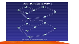
Route Discovery Process
• Source Note initiates path discovery processed by
broadcasting RREQ.
• RREQ is forwarded until it reaches an intermediate
note that has a recent route information about the
desination or till it reaches the destination
• The RREQ uses sequence numbers to ensure that
the routes are loop free & reply contents latest
information only.
8.
AdHov On-Demand DistanceVector Routing( AODV)
Route Reply Process
• When a node forwards a route request packaet to
its neighbours, it also records in its stables the
node from which the first copy of the request came.
• This table is used to construct the reverse path for
the RREQ.
• As the RREP traverses back to the source, the
nodes along the path enter the forward route into
their tables.
9.
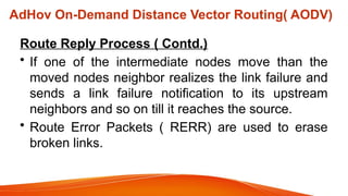
Route Reply Process( Contd.)
• If one of the intermediate nodes move than the
moved nodes neighbor realizes the link failure and
sends a link failure notification to its upstream
neighbors and so on till it reaches the source.
• Route Error Packets ( RERR) are used to erase
broken links.
AdHov On-Demand Distance Vector Routing( AODV)
12.
AdHov On-Demand DistanceVectorRouting( AODV)
Advantages of AODV
• The main adavantage of this protocol is that the
routes are established on demand & destination
sequence numbers are used to find the latest route
to the destination.
• The connection setup delay is lower.
13.
AdHov On-Demand DistanceVectorRouting( AODV)
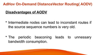
Disadvantages of AODV
• Intermediate nodes can lead to inconstant routes if
the source sequence numbers is very old.
• The periodic beaconing leads to unnessary
bandwidth consumption.
14.
Dynamic Source Routing( DSR )
The two major phases of the protocol are
• Route Discovery
• Route Maintenance
15.
Dynamic Source Routing( DSR )
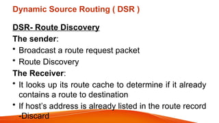
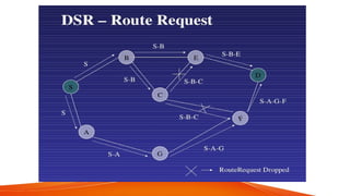
DSR- Route Discovery
The sender:
• Broadcast a route request packet
• Route Discovery
The Receiver:
• It looks up its route cache to determine if it already
contains a route to destination
• If host’s address is already listed in the route record
-Discard
16.
Dynamic Source Routing( DSR )
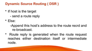
• If host is the target
- send a route reply
• Else:
-Append this host’s address to the route recrd and
re-broadcast.
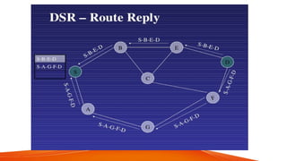
• Route reply is generated when the route request
reaches either destination itself or intermediate
node.
17.
Dynamic Source Routing( DSR )
• When Destination is reached then destination
returns Route Reply with full path
• Source node caches all paths that it receives and
choose shortest path among all the path that it
receives.
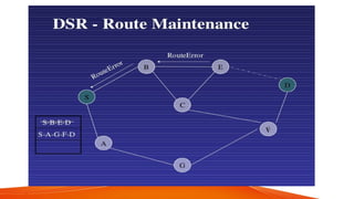
20.
DSR –Route Maintenance
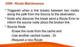
•Triggered when a link breaks between two nodes
along the path from the Source to the destination.
• Node who discover the break send a Route Error to
inform the source node about the broken link.
• Source Node
-Erase the route from the cache and
-Use another cached routes , Or
-Request a new Route
22.
Advantages of DSR:
• A route is established only when it is required and
hence the need to find routes to all other nodes is
eliminated
• The intermediate nodes utilize the route cache
information to reduce the control overhead.
23.
Disadvantages of DSR:
• The route maintenance mechanism does not locally
repair a broken link
• The connection setup delay is higher than in table-
driven protocols
• This routing overhead is directly proportional to the
path length.
24.
Distance –Vector RoutingProtocols :
• A distance-vector routing protocol in data
networks determines the best route for data
packets based on distance.
• Distance-vector routing protocols measure the
distance by the number of touters a packet has
to pass, one router counts as one hop. Some
distance-vector protocols also take into
account network latency and other factors that
influence traffic on a given route.
25.
Distance –Vector RoutingProtocols (Contd.)
• To determine the best route across a network,
routers, on which a distance-vector protocol is
implemented, exchange information with one
another, usually routing tables plus hop counts
for destination networks and possibly other
traffic information.
• Distance-vector routing protocols also require
that a router informs its neighbors of network
topology changes periodically.
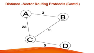
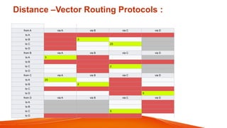
Distance –Vector RoutingProtocols :
from A via A via B via C via D
to A
to B 3
to C 23
to D
from B via A via B via C via D
to A 3
to B
to C 2
to D
from C via A via B via C via D
to A 23
to B 2
to C
to D 5
from D via A via B via C via D
to A
to B
to C 5
to D
28.
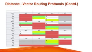
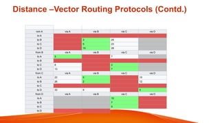
Distance –Vector RoutingProtocols (Contd.)
As we build the routing tables as above, the shortest
path is highlighted in green, and a new shortest path
is highlighted in yellow. Grey columns indicate nodes
that are not neighbors of the current node, and are
therefore not considered as a valid direction in its
table. Red indicates invalid entries in the table since
they refer to distances from a node to itself, or via
itself.
29.
Distance –Vector RoutingProtocols (Contd.)
rom A via A via B via C via D
to A
to B 3 25
to C 5 23
to D 28
from B via A via B via C via D
to A 3 25
to B
to C 26 2
to D 7
from C via A via B via C via D
to A 23 5
to B 26 2
to C
to D 5
from D via A via B via C via D
to A 28
to B 7
to C 5
to D
30.
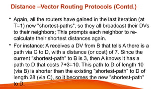
Distance –Vector RoutingProtocols (Contd.)
• Again, all the routers have gained in the last iteration (at
T=1) new "shortest-paths", so they all broadcast their DVs
to their neighbors; This prompts each neighbor to re-
calculate their shortest distances again.
• For instance: A receives a DV from B that tells A there is a
path via C to D, with a distance (or cost) of 7. Since the
current "shortest-path" to B is 3, then A knows it has a
path to D that costs 7+3=10. This path to D of length 10
(via B) is shorter than the existing "shortest-path" to D of
length 28 (via C), so it becomes the new "shortest-path"
to D.
31.
Distance –Vector RoutingProtocols (Contd.)
from A via A via B via C via D
to A
to B 3 25
to C 5 23
to D 10 28
from B via A via B via C via D
to A 3 7
to B
to C 8 2
to D 31 7
from C via A via B via C via D
to A 23 5 33
to B 26 2 12
to C
to D 51 9 5
from D via A via B via C via D
to A 10
to B 7
to C 5
to D
32.
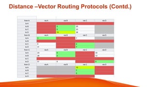
Distance –Vector RoutingProtocols (Contd.)
• This time, only routers A and D have new shortest-
paths for their DVs. So they broadcast their new
DVs to their neighbors: A broadcasts to B and C,
and D broadcasts to C.
• This causes each of the neighbors receiving the
new DVs to re-calculate their shortest paths.
However, since the information from the DVs
doesn't yield any shorter paths than they already
have in their routing tables, then there are no
changes to the routing tables.
33.
Distance –Vector RoutingProtocols (Contd.)
rom A via A via B via C via D
to A
to B 3 25
to C 5 23
to D 10 28
from B via A via B via C via D
to A 3 7
to B
to C 8 2
to D 13 7
from C via A via B via C via D
to A 23 5 15
to B 26 2 12
to C
to D 33 9 5
from D via A via B via C via D
to A 10
to B 7
to C 5
to D
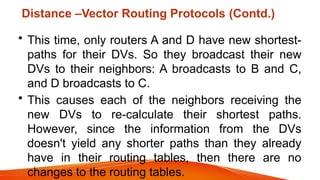
34.
Distance –Vector RoutingProtocols (Contd.)
• None of the routers have any new shortest-paths to
broadcast.
• Therefore, none of the routers receive any new
information that might change their routing tables.
• Hence,The algorithm comes to a stop.
35.
Link State routing
•Also called shortest path first (SPF) forwarding
–Named after Dijkstra’s algorithm (1959) which it uses
to compute routes
• All routers have tables which contain a representation of
the entire network topology
–In the form of lists of routers and information about
each router’s neighbours and the connection between
the two
36.
Link State routing( Contd.)
• LSPs are generated and distributed when:
–A time period passes
–New neighbours connect to the router
–The link cost of a neighbour has changed
–A link to a neighbour has failed (link failure)
–A neighbour has failed (node failure)
37.
Link State routing( Contd.)
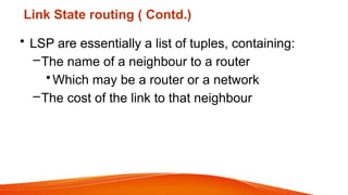
• LSP are essentially a list of tuples, containing:
–The name of a neighbour to a router
•Which may be a router or a network
–The cost of the link to that neighbour
38.
Link State routing( Contd.)
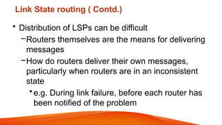
• Distribution of LSPs can be difficult
–Routers themselves are the means for delivering
messages
–How do routers deliver their own messages,
particularly when routers are in an inconsistent
state
•e.g. During link failure, before each router has
been notified of the problem
39.
Dijkstra’s LSR Algorithm
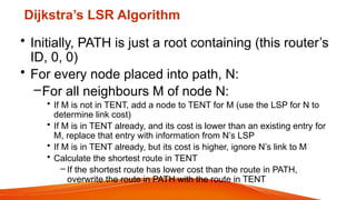
•Initially, PATH is just a root containing (this router’s
ID, 0, 0)
• For every node placed into path, N:
–For all neighbours M of node N:
• If M is not in TENT, add a node to TENT for M (use the LSP for N to
determine link cost)
• If M is in TENT already, and its cost is lower than an existing entry for
M, replace that entry with information from N’s LSP
• If M is in TENT already, but its cost is higher, ignore N’s link to M
• Calculate the shortest route in TENT
– If the shortest route has lower cost than the route in PATH,
overwrite the route in PATH with the route in TENT
40.
Dijkstra’s LSR Algorithm( contd.)
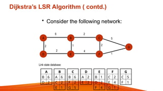
• Consider the following network:
A
D
B
E
C
F
G
2
6
2 4
2
1 2
5
1
Link state database:
A
B 6
D 2
B
A 6
C 2
E 1
C
B 6
F 2
G 5
D
A 2
E 2
E
B 1
D 2
F 4
F
C 2
E 4
G 1
G
C 5
F 1
41.
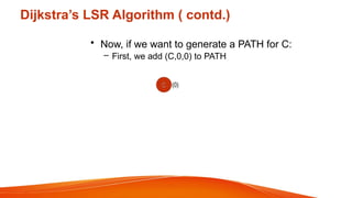
Dijkstra’s LSR Algorithm( contd.)
• Now, if we want to generate a PATH for C:
– First, we add (C,0,0) to PATH
C (0)
42.
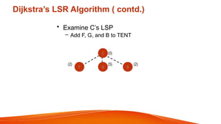
Dijkstra’s LSR Algorithm( contd.)
• Examine C’s LSP
– Add F, G, and B to TENT
C (0)
F G B
(2) (5) (2)
43.
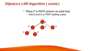
Dijkstra’s LSR Algorithm( contd.)
• Place F in PATH (shown as solid line)
– Add G and E to TENT (adding costs)
C (0)
F G B
(2) (5) (2)
G
E
(3) (6)
44.
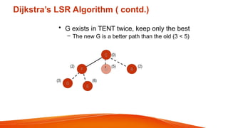
Dijkstra’s LSR Algorithm( contd.)
• G exists in TENT twice, keep only the best
– The new G is a better path than the old (3 < 5)
C (0)
F G B
(2) (5) (2)
G
E
(3) (6)
45.
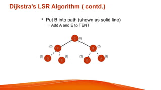
Dijkstra’s LSR Algorithm( contd.)
• Put B into path (shown as solid line)
– Add A and E to TENT
C (0)
F B
(2) (2)
G
E
(3) (6)
A
E
(3) (8)
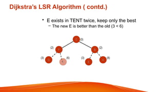
46.
Dijkstra’s LSR Algorithm( contd.)
• E exists in TENT twice, keep only the best
– The new E is better than the old (3 < 6)
C (0)
F B
(2) (2)
G
E
(3) (6)
A
E
(3) (8)
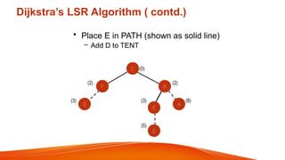
47.
Dijkstra’s LSR Algorithm( contd.)
• Place E in PATH (shown as solid line)
– Add D to TENT
C (0)
F B
(2) (2)
G
(3)
A
E
(3) (8)
D
(5)
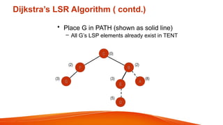
48.
Dijkstra’s LSR Algorithm( contd.)
• Place G in PATH (shown as solid line)
– All G’s LSP elements already exist in TENT
C (0)
F B
(2) (2)
G
(3)
A
E
(3) (8)
D
(5)
49.
Dijkstra’s LSR Algorithm( contd.)
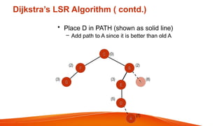
• Place D in PATH (shown as solid line)
– Add path to A since it is better than old A
C (0)
F B
(2) (2)
G
(3)
A
E
(3) (8)
D
(5)
A
(7)
50.
Dijkstra’s LSR Algorithm( contd.)
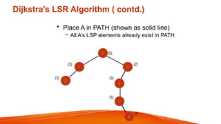
• Place A in PATH (shown as solid line)
– All A’s LSP elements already exist in PATH
C (0)
F B
(2) (2)
G
(3)
E
(3)
D
(5)
A
(7)
51.
Dijkstra’s LSR Algorithm( contd.)
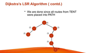
• We are done since all routes from TENT
were placed into PATH
C (0)
F B
(2) (2)
G
(3)
E
(3)
D
(5)
A
(7)
52.
Dijkstra’s LSR Algorithm( contd.)
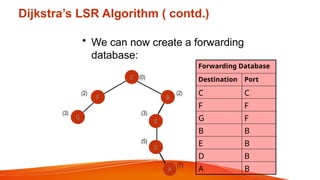
• We can now create a forwarding
database:
C (0)
F B
(2) (2)
G
(3)
E
(3)
D
(5)
A
(7)
Forwarding Database
Destination Port
C C
F F
G F
B B
E B
D B
A B
53.
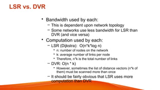
LSR vs. DVR
•Bandwidth used by each:
– This is dependent upon network topology
– Some networks use less bandwidth for LSR than
DVR (and vice versa)
• Computation used by each:
– LSR (Dijkstra): O(n*k*log n)
• n: number of nodes on the network
• k: average number of links per node
• Therefore, n*k is the total number of links
– DVR: O(n * k)
• However, sometimes the list of distance vectors (n*k of
them) must be scanned more than once
– It should be fairly obvious that LSR uses more
computation than DVR
54.
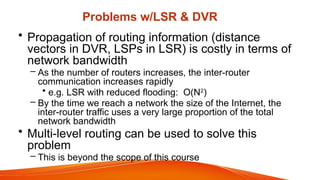
Problems w/LSR &DVR
• Propagation of routing information (distance
vectors in DVR, LSPs in LSR) is costly in terms of
network bandwidth
– As the number of routers increases, the inter-router
communication increases rapidly
• e.g. LSR with reduced flooding: O(N2
)
– By the time we reach a network the size of the Internet, the
inter-router traffic uses a very large proportion of the total
network bandwidth
• Multi-level routing can be used to solve this
problem
– This is beyond the scope of this course
CONCLUSION AND FUTURESCOPE
CONCLUSION
• Considering the executed simulations and the gained outcomes we can conclude that the most efficient
protocol is EIGRP because uses a less complicated algorithm than the one OSPF does; this one is
very well scaled on the middle-sized networks and well on the big-sized networks, while OSPF is very
well scaled both on the middle-sized and big-sized networks, the latter computing the shortest route.
Each router will announce in the entire network the routing table and each router using this one will
compute the topology of the entire network, requesting very big resources and higher costs comparing
to EIGRP. The last protocol that could be used for routing a topology is RIP because its time is not very
good, therefore it will generate delays in the network.
• From the analysis made and the response times obtained, we can conclude that there are differences
between the used routing protocols. These differences are generated by the used algorithms that
introduce the delays in the execution of some services. We consider that a viable software for the
network simulation is Packet Tracer. This software allows us to design and simulate virtual networks,
by using them we can obtain a traffic decongestion and at the same time we can strengthen the
network security.
64.
CONCLUSION AND FUTURESCOPE
FUTURE SCOPE
The only varying parameter in our analysis, aside from routing protocol in fact , was the dimensions of the
topology . Improvement or future works for this project can include adding metrics on interfaces like cost,
bandwidth, distance, Bit Error Rate (BER), and delay. Furthermore, various network topologies (in terms of
size, routers and links used) are often implemented for comparison of performance between these routing
protocols. Since OSPF is that the most complex routing protocol, longer might be spent on analyzing it to
seek out the worth of parameters that require to be set so as for it to perform optimally. Another possibility
is to implement real network topologies used, perhaps during a university campus a corporation office, or a
bigger network.