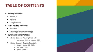
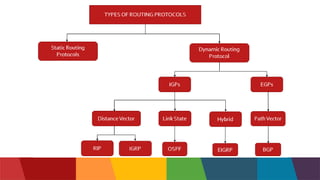
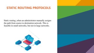
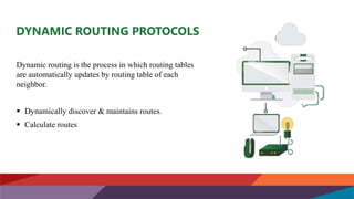
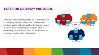
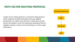
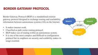
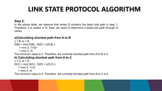
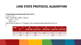
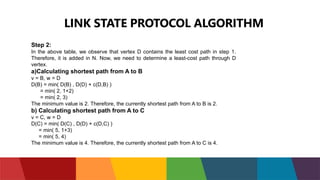
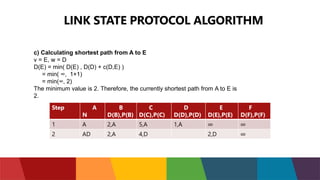
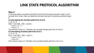
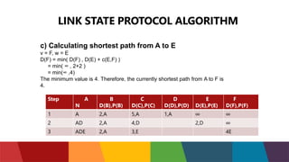
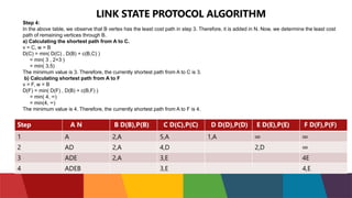
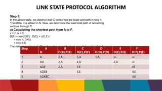
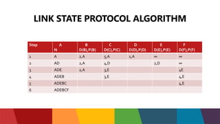
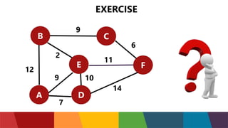
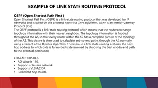
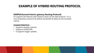
The document discusses different routing protocols used in computer networks. It begins with an introduction to routing protocols and their purpose of communicating between source and destination networks by updating routing tables. It then categorizes routing protocols as static or dynamic and discusses examples in each category. For dynamic routing protocols, it further divides them into interior gateway protocols used within an autonomous system and exterior gateway protocols used between autonomous systems. Specific dynamic interior routing protocols discussed in detail include distance vector protocols like RIP and link state protocols like OSPF.

1. INTERNET ARCHITECTURE
AND PROTOCOLS (IT-313)
PRESENTATION
TOPIC:
ROUTING PROTOCOLS

2. GROUP PRESENTATION
GROUP #5 (SECTION B)
PRESENTED TO: MADAM SARA SARWAR
PRESENTERS :
MAEDA QAISAR (19011556-078)
FAIZA (19011556-176)
ALISHBA SHAHBAZ (19011556-043)

3. TABLE OF CONTENTS
• Routing Protocols
• Definition
• Metrices
• Categorization
• Static Routing Protocols
• Definition
• Advantages and Disadvantages
• Dynamic Routing Protocols
• Exterior Gateway Routing Protocols
• Path Vector Routing Protocol (BGP)
• Interior Gateway Routing Protocols
• Distance Vector (RIP, IGRP)
• Link State (OSPF)
• Hybrid (EIGRP)

4. ROUTING PROTOCOLS
Routing protocols are the set of rules used by the routers
to communicate between source & destination. They do
not move the information source to destination only
update the routing table. Each protocol has its own
algorithm to choose the best path.

5. METRICES BY ROUTING PROTOCOLS
• Number of network layer devices along with the path (hop count)
• Bandwidth
• Delay
• Load
• MTU
• Cost
Routing protocols store the result of these metrices in routing table.

7. STATIC ROUTING PROTOCOLS
Static routing ,when an administrator manually assigns
the path from source to destination network. This is
feasible in small networks, but not in large networks.

8. ADVANTAGES & DISADVANTAGES
Advantages:
• No overhead on router CPU.
• No bandwidth usage between links.
• Security (only administrator add routes.)
Disadvantages:
• All link will be down on a link failure.
• Not practical on large networks.
• Administrator must update all routes.

9. DYNAMIC ROUTING PROTOCOLS
Dynamic routing is the process in which routing tables
are automatically updates by routing table of each
neighbor.
 Dynamically discover & maintains routes.
 Calculate routes

10. ADVANTAGES & DISADVANTAGES
Advantages:
• Less work in maintaining the configuration when adding &
deleting networks.
• Protocols automatically react to the topology changes.
• Configuration is less-prone.
Disadvantages:
• Routers resource are used
• More administrator knowledge is required for configuration.

11. EXTERIOR GATEWAY PROTOCOL
Exterior Gateway Protocol (EGP) is a protocol for
exchanging routing information between two
neighbor gateway hosts (each with its own router)
in a network of autonomous systems. EGP is
commonly used between hosts on the Internet to
exchange routing table information.

12. PATH VECTOR ROUTING PROTOCOL
A path-vector routing protocol is a network routing protocol
which maintains the path information that gets updated
dynamically. In a path vector protocol, a router does not just
receive the distance vector for a particular destination from its
neighbor; instead, a node receives the distance as well as path
information.

13. Border Gateway Protocol (BGP) is a standardized exterior
gateway protocol designed to exchange routing and reachability
information between autonomous systems (AS) on the Internet.
• It makes internet work.
• Classified as path vector routing protocol.
• BGP makes use of routing within an autonomous system.
• It is one of the most complex and Difficult to configuration
protocol but its emphasis on security and scalability makes its
usage essential.
BORDER GATEWAY PROTOCOL

14. DISTANCE VECTOR ROUTING PROTOCOL
Distance vector routing protocols use distance to determine the best path to a remote
network.
The distance is usually the number of hops (routers) to the destination network.
Distance vector protocols send complete routing table to each neighbor (a neighbor is
directly connected router that runs the same routing protocol)
RIPV1 and RIPV2 are examples of distance vector routing protocols.

15. DISTANCE VECTOR ROUTING PROTOCOL
Consider
• There is a network consisting of 4 routers.
• The weights are mentioned on the edges.
• Weights could be distances or costs or delays

16. DISTANCE VECTOR ROUTING PROTOCOL ALGORITHM
Step-01:
Each router prepares its routing table using its local knowledge.
Routing table prepared by each router is shown below-
Destination Distance Next HOP
A 0 A
B 2 B
C ∞ –
D 1 D
Destination Distance Next HOP
A 2 A
B 0 B
C 3 C
D 7 D
At Router A- AT Router B-

17. DISTANCE VECTOR ROUTING PROTOCOL ALGORITHM
Step 1
Destination Distance Next Hop
A ∞ –
B 3 B
C 0 C
D 11 D
Destination Distance Next Hop
A 1 A
B 7 B
C 11 C
D 0 D
At Router C- AT Router D-

18. DISTANCE VECTOR ROUTING PROTOCOL ALGORITHM
Step-02:
Each router exchanges its distance vector obtained in Step-01 with its neighbors.
After exchanging the distance vectors, each router prepares a new routing table.
This is shown below-
At Router A-
Router A receives distance vectors from its neighbors B and D.
Router A prepares a new routing table as-

19. DISTANCE VECTOR ROUTING PROTOCOL ALGORITHM
Cost of reaching destination B from router A = min { 2+0 , 1+7 } = 2 via B.
Cost of reaching destination C from router A = min { 2+3 , 1+11 } = 5 via B.
Cost of reaching destination D from router A = min { 2+7 , 1+0 } = 1 via D.
Thus, the new routing table at router A is-
Destination Distance Next Hop
A 0 A
B 2 B
C 5 B
D 1 D

20. DISTANCE VECTOR ROUTING PROTOCOL ALGORITHM
At Router B-
Router B receives distance vectors from its neighbors A, C and D.
Router B prepares a new routing table as-
•Cost of reaching destination A from router B = min { 2+0 , 3+∞ , 7+1 } = 2 via A.
•Cost of reaching destination C from router B = min { 2+∞ , 3+0 , 7+11 } = 3 via C.
•Cost of reaching destination D from router B = min { 2+1 , 3+11 , 7+0 } = 3 via A

21. DISTANCE VECTOR ROUTING PROTOCOL ALGORITHM
Thus, the new routing table at router B is-
At Router C-
•Router C receives distance vectors from its
neighbors B and D.
•Router C prepares a new routing table as
Destination Distance Next Hop
A 2 A
B 0 B
C 3 C
D 3 A

22. DISTANCE VECTOR ROUTING PROTOCOL ALGORITHM
• Cost of reaching destination A from router C = min { 3+2 , 11+1 } = 5 via B.
• Cost of reaching destination B from router C = min { 3+0 , 11+7 } = 3 via B.
• Cost of reaching destination D from router C = min { 3+7 , 11+0 } = 10 via B
• Thus, the new routing table at router C is-
Destination Distance Next Hop
A 5 B
B 3 B
C 0 C
D 10 B

23. DISTANCE VECTOR ROUTING PROTOCOL ALGORITHM
At Router D
•Router D receives distance vectors from its neighbors A, B and C.
•Router D prepares a new routing table as-
•Cost of reaching destination A from router D = min { 1+0 , 7+2 , 11+∞ } = 1 via A.
•Cost of reaching destination B from router D = min { 1+2 , 7+0 , 11+3 } = 3 via A.
•Cost of reaching destination C from router D = min { 1+∞ , 7+3 , 11+0 } = 10 via B

24. DISTANCE VECTOR ROUTING PROTOCOL ALGORITHM
Thus, the new routing table at router D is-
Step-03:
• Each router exchanges its distance vector obtained in Step-02 with its neighboring routers
• After exchanging the distance vectors, each router prepares a new routing table
At Router A-
• Router A receives distance vectors from its neighbors B and D.
• Router A prepares a new routing table as
Destination Distance Next Hop
A 1 A
B 3 A
C 10 B
D 0 D

25. DISTANCE VECTOR ROUTING PROTOCOL ALGORITHM
• Cost of reaching destination B from router A = min { 2+0 , 1+3 } = 2 via B
• Cost of reaching destination C from router A = min { 2+3 , 1+10 } = 5 via B
• Cost of reaching destination D from router A = min { 2+3 , 1+0 } = 1 via D
• Thus, the new routing table at router A is-
Destination Distance Next Hop
A 0 A
B 2 B
C 5 B
D 1 D

26. DISTANCE VECTOR ROUTING PROTOCOL ALGORITHM
• Router B receives distance vectors from its neighbors A, C and D.
• Router B prepares a new routing table as-
• Cost of reaching destination A from router B = min { 2+0 , 3+5 , 3+1 } = 2 via A.
• Cost of reaching destination C from router B = min { 2+5 , 3+0 , 3+10 } = 3 via
• Cost of reaching destination D from router B = min { 2+1 , 3+10 , 3+0 } = 3 via A
Destination Distance Next Hop
A 2 A
B 0 B
C 3 C
D 3 A

27. DISTANCE VECTOR ROUTING PROTOCOL ALGORITHM
Thus, the new routing table at router B is-
At Router C-
• Router C receives distance vectors from its neighbors B and D.
• Router C prepares a new routing table as
Destination Distance Next Hop
A 2 A
B 0 B
C 3 C
D 3 A

28. DISTANCE VECTOR ROUTING PROTOCOL ALGORITHM
• Cost of reaching destination A from router C = min { 3+2 , 10+1 } = 5 via B.
• Cost of reaching destination B from router C = min { 3+0 , 10+3 } = 3 via B.
• Cost of reaching destination D from router C = min { 3+3 , 10+0 } = 6 via B.
• Thus, the new routing table at router C is-
• At Router D-
• Router D receives distance vectors from its neighbors A, B
• and C
• Router D prepares a new
routing table as-
Destination Distance Next Hop
A 5 B
B 3 B
C 0 C
D 6 B

29. DISTANCE VECTOR ROUTING PROTOCOL ALGORITHM
• Cost of reaching destination A from router D = min { 1+0 , 3+2 , 10+5 } = 1 via A.
• Cost of reaching destination B from router D = min { 1+2 , 3+0 , 10+3 } = 3 via A.
• Cost of reaching destination C from router D = min { 1+5 , 3+3 , 10+0 } = 6 via A
• Thus, the new routing table at router D is
• These will be the final routing tables at each router.
Destination Distance Next Hop
A 1 A
B 3 A
C 6 A
D 0 D

30. DISTANCE VECTOR ROUTING PROTOCOL ALGORITHM
FINAL ROUTING TABLE:
Information stored at node
A B C D
A 0 2 5 1
B
2 0 3 3
C
5 3 0 6
D 1 3 6 0

31. LINK STATE PROTOCOL
Link state routing protocols are the second type of dynamic routing protocols.
They have the same basic purpose as distance vector protocols, to find a best path
to a destination, but use different methods to do so. Unlike distance vector
protocols, link state protocols don't advertise the entire routing table. Instead,
they advertise information about a network topology (directly connected links,
neighboring routers...), so that in the end all routers running a link state protocol
have the same topology database.
OSPF are the examples of link state routing protocols.

32. LINK STATE PROTOCOL ALGORITHM
Initialization
N = {A} // A is a root node.
for all nodes v
if v adjacent to A
then D(v) = c( A, v)
else D(v) = infinity
loop
find w not in N such that D(w) is a minimum.
Add w to N
Update D(v) for all v adjacent to w and not in N:
D(v) = min(D(v) , D(w) + c( w, v))
Until all nodes in N

33. Explain with the help
of this graph
A
E
D
C
B
F
1
3
2
2
5
1
1
2
5

34. LINK STATE PROTOCOL ALGORITHM
Step 1:
The first step is an initialization step. The currently known least cost path
from A to its directly attached neighbors, B, C, D are 2,5,1 respectively. The
cost from A to B is set to 2, from A to D is set to 1 and from A to C is set to 5.
The cost from A to E and F are set to infinity as they are not directly linked to
A.
Step A
N
B
D(B),P(B
)
C
D(C),P(C
)
D
D(D),P(D
)
E
D(E),P(E)
F
D(F),P(F)
1 A 2,A 5,A 1,A ∞ ∞

35. LINK STATE PROTOCOL ALGORITHM
Step 2:
In the above table, we observe that vertex D contains the least cost path in step 1.
Therefore, it is added in N. Now, we need to determine a least-cost path through D
vertex.
a)Calculating shortest path from A to B
v = B, w = D
D(B) = min( D(B) , D(D) + c(D,B) )
= min( 2, 1+2)>
= min( 2, 3)
The minimum value is 2. Therefore, the currently shortest path from A to B is 2
b) Calculating shortest path from A to C
v = C, w = D
D(C) = min( D(C) , D(D) + c(D,C) )
= min( 5, 1+3)
= min( 5, 4)
The minimum value is 4. Therefore, the currently shortest path from A to C is 4.

36. LINK STATE PROTOCOL ALGORITHM
c) Calculating shortest path from A to E
v = E, w = D
D(E) = min( D(E) , D(D) + c(D,E) )
= min( ∞, 1+1)
= min(∞, 2)
The minimum value is 2. Therefore, the currently shortest path from A to E is
2.
Step A
N
B
D(B),P(B)
C
D(C),P(C)
D
D(D),P(D)
E
D(E),P(E)
F
D(F),P(F)
1 A 2,A 5,A 1,A ∞ ∞
2 AD 2,A 4,D 2,D ∞

37. LINK STATE PROTOCOL ALGORITHM
Step 2:
In the above table, we observe that vertex D contains the least cost path in step 1.
Therefore, it is added in N. Now, we need to determine a least-cost path through D
vertex.
a)Calculating shortest path from A to B
v = B, w = D
D(B) = min( D(B) , D(D) + c(D,B) )
= min( 2, 1+2)
= min( 2, 3)
The minimum value is 2. Therefore, the currently shortest path from A to B is 2.
b) Calculating shortest path from A to C
v = C, w = D
D(C) = min( D(C) , D(D) + c(D,C) )
= min( 5, 1+3)
= min( 5, 4)
The minimum value is 4. Therefore, the currently shortest path from A to C is 4.

38. LINK STATE PROTOCOL ALGORITHM
c) Calculating shortest path from A to E
v = E, w = D
D(E) = min( D(E) , D(D) + c(D,E) )
= min( ∞, 1+1)
= min(∞, 2)
The minimum value is 2. Therefore, the currently shortest path from A to E is
2.
Step A
N
B
D(B),P(B)
C
D(C),P(C)
D
D(D),P(D)
E
D(E),P(E)
F
D(F),P(F)
1 A 2,A 5,A 1,A ∞ ∞
2 AD 2,A 4,D 2,D ∞

39. LINK STATE PROTOCOL ALGORITHM
Step 3:
In the above table, we observe that both E and B have the least cost path in step 2. Let's
consider the E vertex. Now, we determine the least cost path of remaining vertices through
E.
a) Calculating the shortest path from A to B.
v = B, w = E
D(B) = min( D(B) , D(E) + c(E,B) )
= min( 2 , 2+ ∞ )
= min( 2, ∞)
The minimum value is 2. Therefore, the currently shortest path from A to B is 2.
b) Calculating shortest path from A to C
v = C, w = E
D(C) = min( D(C) , D(E) + c(E,C) )
= min( 4 , 2+1 )
= min( 4,3)
The minimum value is 3. Therefore, the currently shortest path from A to C is 3.

40. LINK STATE PROTOCOL ALGORITHM
c) Calculating shortest path from A to E
v = F, w = E
D(F) = min( D(F) , D(E) + c(E,F) )
= min( ∞ , 2+2 )
= min(∞ ,4)
The minimum value is 4. Therefore, the currently shortest path from A to F is
4.
Step A
N
B
D(B),P(B)
C
D(C),P(C)
D
D(D),P(D)
E
D(E),P(E)
F
D(F),P(F)
1 A 2,A 5,A 1,A ∞ ∞
2 AD 2,A 4,D 2,D ∞
3 ADE 2,A 3,E 4E

41. LINK STATE PROTOCOL ALGORITHM
Step 4:
In the above table, we observe that B vertex has the least cost path in step 3. Therefore, it is added in N. Now, we determine the least cost
path of remaining vertices through B.
a) Calculating the shortest path from A to C.
v = C, w = B
D(C) = min( D(C) , D(B) + c(B,C) )
= min( 3 , 2+3 )
= min( 3,5)
The minimum value is 3. Therefore, the currently shortest path from A to C is 3.
b) Calculating shortest path from A to F
v = F, w = B
D(F) = min( D(F) , D(B) + c(B,F) )
= min( 4, ∞)
= min(4, ∞)
The minimum value is 4. Therefore, the currently shortest path from A to F is 4.
Step A N B D(B),P(B) C D(C),P(C) D D(D),P(D) E D(E),P(E) F D(F),P(F)
1 A 2,A 5,A 1,A ∞ ∞
2 AD 2,A 4,D 2,D ∞
3 ADE 2,A 3,E 4E
4 ADEB 3,E 4,E

42. LINK STATE PROTOCOL ALGORITHM
Step 5:
In the above table, we observe that C vertex has the least cost path in step 4.
Therefore, it is added in N. Now, we determine the least cost path of remaining
vertices through C.
a) Calculating the shortest path from A to F.
v = F, w = C
D(F) = min( D(F) , D(C) + c(C,F) )
= min( 4, 3+5)
= min(4,8)
The minimum value is 4. Therefore, the currently shortest path from A to F is 4.
Step A
N
B
D(B),P(B)
C
D(C),P(C)
D
D(D),P(D)
E
D(E),P(E)
F
D(F),P(F)
1 A 2,A 5,A 1,A ∞ ∞
2 AD 2,A 4,D 2,D ∞
3 ADE 2,A 3,E 4E
4 ADEB 3,E 4,E
5 ADEBC 4,E

43. LINK STATE PROTOCOL ALGORITHM
Step A
N
B
D(B),P(B)
C
D(C),P(C)
D
D(D),P(D)
E
D(E),P(E)
F
D(F),P(F)
1 A 2,A 5,A 1,A ∞ ∞
2 AD 2,A 4,D 2,D ∞
3 ADE 2,A 3,E 4E
4 ADEB 3,E 4,E
5 ADEBC 4,E
6 ADEBCF

44. EXERCISE
A
E
D
C
B
F
7
9
2
12
11
9
14
6
10

45. EXAMPLE OF LINK STATE ROUTING PROTOCOL
OSPF (Open Shortest Path First )
Open Shortest Path First (OSPF) is a link-state routing protocol that was developed for IP
networks and is based on the Shortest Path First (SPF) algorithm. OSPF is an Interior Gateway
Protocol (IGP).
The OSPF protocol is a link-state routing protocol, which means that the routers exchange
topology information with their nearest neighbors. The topology information is flooded
throughout the AS, so that every router within the AS has a complete picture of the topology
of the AS. This picture is then used to calculate end-to-end paths through the AS, normally
using a variant of the Dijkstra algorithm. Therefore, in a link-state routing protocol, the next
hop address to which data is forwarded is determined by choosing the best end-to-end path
to the eventual destination
CHARACTERISTICS:
• AD value is 110.
• Supports classless network.
• Supports VLSM/CIDR
• unlimited hop counts.

46. HYBRID ROUTING PROTOCOL
A Hybrid Routing protocol has the advantages of both Distance Vector and Link
State Routing protocols and merges them into a new protocol. Typically, hybrid routing
protocols are based on a Distance Vector protocol but contain many of the features
and advantages of Link State Routing protocols. Example: EIGRP (Enhanced Interior
Gateway Routing Protocol).
Hybrid Routing Protocol (HRP) Requires less memory and processing power than LSRP
EIGRP are examples of hybrid routing protocols.

47. EXAMPLE OF HYBIRD ROUTING PROTOCOL
EIGRP(Enhanced Interior gateway Routing Protocol)
It’s supports the features both distance vector & link state protocol. It is a
cisco proprietary protocol. By default, bandwidth & delay are the activated
metrics.
CHARACTERISTICS: -
• Supports classless network
• Supports VLSM/CIDR.
• It supports trigger updates.