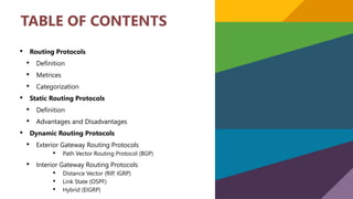
INTERNET ARCHITECTURE
AND PROTOCOLS (IT-313)
PRESENTATION
TOPIC:
ROUTING PROTOCOLS
GROUP PRESENTATION
GROUP #5 (SECTION B)
PRESENTED TO: MADAM SARA SARWAR
PRESENTERS :
MAEDA QAISAR (19011556-078)
FAIZA (19011556-176)
ALISHBA SHAHBAZ (19011556-043)
TABLE OF CONTENTS
• Routing Protocols
• Definition
• Metrices
• Categorization
• Static Routing Protocols
• Definition
• Advantages and Disadvantages
• Dynamic Routing Protocols
• Exterior Gateway Routing Protocols
• Path Vector Routing Protocol (BGP)
• Interior Gateway Routing Protocols
• Distance Vector (RIP, IGRP)
• Link State (OSPF)
• Hybrid (EIGRP)
ROUTING PROTOCOLS
Routing protocols are the set of rules used by the routers
to communicate between source & destination. They do
not move the information source to destination only
update the routing table. Each protocol has its own
algorithm to choose the best path.
METRICES BY ROUTING PROTOCOLS
• Number of network layer devices along with the path (hop count)
• Bandwidth
• Delay
• Load
• MTU
• Cost
Routing protocols store the result of these metrices in routing table.
STATIC ROUTING PROTOCOLS
Static routing ,when an administrator manually assigns
the path from source to destination network. This is
feasible in small networks, but not in large networks.
ADVANTAGES & DISADVANTAGES
Advantages:
• No overhead on router CPU.
• No bandwidth usage between links.
• Security (only administrator add routes.)
Disadvantages:
• All link will be down on a link failure.
• Not practical on large networks.
• Administrator must update all routes.
DYNAMIC ROUTING PROTOCOLS
Dynamic routing is the process in which routing tables
are automatically updates by routing table of each
neighbor.
 Dynamically discover & maintains routes.
 Calculate routes
ADVANTAGES & DISADVANTAGES
Advantages:
• Less work in maintaining the configuration when adding &
deleting networks.
• Protocols automatically react to the topology changes.
• Configuration is less-prone.
Disadvantages:
• Routers resource are used
• More administrator knowledge is required for configuration.
EXTERIOR GATEWAY PROTOCOL
Exterior Gateway Protocol (EGP) is a protocol for
exchanging routing information between two
neighbor gateway hosts (each with its own router)
in a network of autonomous systems. EGP is
commonly used between hosts on the Internet to
exchange routing table information.
PATH VECTOR ROUTING PROTOCOL
A path-vector routing protocol is a network routing protocol
which maintains the path information that gets updated
dynamically. In a path vector protocol, a router does not just
receive the distance vector for a particular destination from its
neighbor; instead, a node receives the distance as well as path
information.
Border Gateway Protocol (BGP) is a standardized exterior
gateway protocol designed to exchange routing and reachability
information between autonomous systems (AS) on the Internet.
• It makes internet work.
• Classified as path vector routing protocol.
• BGP makes use of routing within an autonomous system.
• It is one of the most complex and Difficult to configuration
protocol but its emphasis on security and scalability makes its
usage essential.
BORDER GATEWAY PROTOCOL
LINK STATE PROTOCOL
Link state routing protocols are the second type of dynamic routing protocols.
They have the same basic purpose as distance vector protocols, to find a best path
to a destination, but use different methods to do so. Unlike distance vector
protocols, link state protocols don't advertise the entire routing table. Instead,
they advertise information about a network topology (directly connected links,
neighboring routers...), so that in the end all routers running a link state protocol
have the same topology database.
OSPF are the examples of link state routing protocols.
LINK STATE PROTOCOL ALGORITHM
Initialization
N = {A} // A is a root node.
for all nodes v
if v adjacent to A
then D(v) = c( A, v)
else D(v) = infinity
loop
find w not in N such that D(w) is a minimum.
Add w to N
Update D(v) for all v adjacent to w and not in N:
D(v) = min(D(v) , D(w) + c( w, v))
Until all nodes in N
Explain with the help
of this graph
A
E
D
C
B
F
1
3
2
2
5
1
1
2
5
LINK STATE PROTOCOL ALGORITHM
Step 1:
The first step is an initialization step. The currently known least cost path
from A to its directly attached neighbors, B, C, D are 2,5,1 respectively. The
cost from A to B is set to 2, from A to D is set to 1 and from A to C is set to 5.
The cost from A to E and F are set to infinity as they are not directly linked to
A.
Step A
N
B
D(B),P(B
)
C
D(C),P(C
)
D
D(D),P(D
)
E
D(E),P(E)
F
D(F),P(F)
1 A 2,A 5,A 1,A ∞ ∞
LINK STATE PROTOCOL ALGORITHM
Step 2:
In the above table, we observe that vertex D contains the least cost path in step 1.
Therefore, it is added in N. Now, we need to determine a least-cost path through D
vertex.
a)Calculating shortest path from A to B
v = B, w = D
D(B) = min( D(B) , D(D) + c(D,B) )
= min( 2, 1+2)>
= min( 2, 3)
The minimum value is 2. Therefore, the currently shortest path from A to B is 2
b) Calculating shortest path from A to C
v = C, w = D
D(C) = min( D(C) , D(D) + c(D,C) )
= min( 5, 1+3)
= min( 5, 4)
The minimum value is 4. Therefore, the currently shortest path from A to C is 4.
LINK STATE PROTOCOL ALGORITHM
c) Calculating shortest path from A to E
v = E, w = D
D(E) = min( D(E) , D(D) + c(D,E) )
= min( ∞, 1+1)
= min(∞, 2)
The minimum value is 2. Therefore, the currently shortest path from A to E is
2.
Step A
N
B
D(B),P(B)
C
D(C),P(C)
D
D(D),P(D)
E
D(E),P(E)
F
D(F),P(F)
1 A 2,A 5,A 1,A ∞ ∞
2 AD 2,A 4,D 2,D ∞
LINK STATE PROTOCOL ALGORITHM
Step 2:
In the above table, we observe that vertex D contains the least cost path in step 1.
Therefore, it is added in N. Now, we need to determine a least-cost path through D
vertex.
a)Calculating shortest path from A to B
v = B, w = D
D(B) = min( D(B) , D(D) + c(D,B) )
= min( 2, 1+2)
= min( 2, 3)
The minimum value is 2. Therefore, the currently shortest path from A to B is 2.
b) Calculating shortest path from A to C
v = C, w = D
D(C) = min( D(C) , D(D) + c(D,C) )
= min( 5, 1+3)
= min( 5, 4)
The minimum value is 4. Therefore, the currently shortest path from A to C is 4.
LINK STATE PROTOCOL ALGORITHM
c) Calculating shortest path from A to E
v = E, w = D
D(E) = min( D(E) , D(D) + c(D,E) )
= min( ∞, 1+1)
= min(∞, 2)
The minimum value is 2. Therefore, the currently shortest path from A to E is
2.
Step A
N
B
D(B),P(B)
C
D(C),P(C)
D
D(D),P(D)
E
D(E),P(E)
F
D(F),P(F)
1 A 2,A 5,A 1,A ∞ ∞
2 AD 2,A 4,D 2,D ∞
LINK STATE PROTOCOL ALGORITHM
Step 3:
In the above table, we observe that both E and B have the least cost path in step 2. Let's
consider the E vertex. Now, we determine the least cost path of remaining vertices through
E.
a) Calculating the shortest path from A to B.
v = B, w = E
D(B) = min( D(B) , D(E) + c(E,B) )
= min( 2 , 2+ ∞ )
= min( 2, ∞)
The minimum value is 2. Therefore, the currently shortest path from A to B is 2.
b) Calculating shortest path from A to C
v = C, w = E
D(C) = min( D(C) , D(E) + c(E,C) )
= min( 4 , 2+1 )
= min( 4,3)
The minimum value is 3. Therefore, the currently shortest path from A to C is 3.
LINK STATE PROTOCOL ALGORITHM
c) Calculating shortest path from A to E
v = F, w = E
D(F) = min( D(F) , D(E) + c(E,F) )
= min( ∞ , 2+2 )
= min(∞ ,4)
The minimum value is 4. Therefore, the currently shortest path from A to F is
4.
Step A
N
B
D(B),P(B)
C
D(C),P(C)
D
D(D),P(D)
E
D(E),P(E)
F
D(F),P(F)
1 A 2,A 5,A 1,A ∞ ∞
2 AD 2,A 4,D 2,D ∞
3 ADE 2,A 3,E 4E
LINK STATE PROTOCOL ALGORITHM
Step 4:
In the above table, we observe that B vertex has the least cost path in step 3. Therefore, it is added in N. Now, we determine the least cost
path of remaining vertices through B.
a) Calculating the shortest path from A to C.
v = C, w = B
D(C) = min( D(C) , D(B) + c(B,C) )
= min( 3 , 2+3 )
= min( 3,5)
The minimum value is 3. Therefore, the currently shortest path from A to C is 3.
b) Calculating shortest path from A to F
v = F, w = B
D(F) = min( D(F) , D(B) + c(B,F) )
= min( 4, ∞)
= min(4, ∞)
The minimum value is 4. Therefore, the currently shortest path from A to F is 4.
Step A N B D(B),P(B) C D(C),P(C) D D(D),P(D) E D(E),P(E) F D(F),P(F)
1 A 2,A 5,A 1,A ∞ ∞
2 AD 2,A 4,D 2,D ∞
3 ADE 2,A 3,E 4E
4 ADEB 3,E 4,E
LINK STATE PROTOCOL ALGORITHM
Step 5:
In the above table, we observe that C vertex has the least cost path in step 4.
Therefore, it is added in N. Now, we determine the least cost path of remaining
vertices through C.
a) Calculating the shortest path from A to F.
v = F, w = C
D(F) = min( D(F) , D(C) + c(C,F) )
= min( 4, 3+5)
= min(4,8)
The minimum value is 4. Therefore, the currently shortest path from A to F is 4.
Step A
N
B
D(B),P(B)
C
D(C),P(C)
D
D(D),P(D)
E
D(E),P(E)
F
D(F),P(F)
1 A 2,A 5,A 1,A ∞ ∞
2 AD 2,A 4,D 2,D ∞
3 ADE 2,A 3,E 4E
4 ADEB 3,E 4,E
5 ADEBC 4,E
LINK STATE PROTOCOL ALGORITHM
Step A
N
B
D(B),P(B)
C
D(C),P(C)
D
D(D),P(D)
E
D(E),P(E)
F
D(F),P(F)
1 A 2,A 5,A 1,A ∞ ∞
2 AD 2,A 4,D 2,D ∞
3 ADE 2,A 3,E 4E
4 ADEB 3,E 4,E
5 ADEBC 4,E
6 ADEBCF
EXERCISE
A
E
D
C
B
F
7
9
2
12
11
9
14
6
10
EXAMPLE OF LINK STATE ROUTING PROTOCOL
OSPF (Open Shortest Path First )
Open Shortest Path First (OSPF) is a link-state routing protocol that was developed for IP
networks and is based on the Shortest Path First (SPF) algorithm. OSPF is an Interior Gateway
Protocol (IGP).
The OSPF protocol is a link-state routing protocol, which means that the routers exchange
topology information with their nearest neighbors. The topology information is flooded
throughout the AS, so that every router within the AS has a complete picture of the topology
of the AS. This picture is then used to calculate end-to-end paths through the AS, normally
using a variant of the Dijkstra algorithm. Therefore, in a link-state routing protocol, the next
hop address to which data is forwarded is determined by choosing the best end-to-end path
to the eventual destination
CHARACTERISTICS:
• AD value is 110.
• Supports classless network.
• Supports VLSM/CIDR
• unlimited hop counts.
HYBRID ROUTING PROTOCOL
A Hybrid Routing protocol has the advantages of both Distance Vector and Link
State Routing protocols and merges them into a new protocol. Typically, hybrid routing
protocols are based on a Distance Vector protocol but contain many of the features
and advantages of Link State Routing protocols. Example: EIGRP (Enhanced Interior
Gateway Routing Protocol).
Hybrid Routing Protocol (HRP) Requires less memory and processing power than LSRP
EIGRP are examples of hybrid routing protocols.
EXAMPLE OF HYBIRD ROUTING PROTOCOL
EIGRP(Enhanced Interior gateway Routing Protocol)
It’s supports the features both distance vector & link state protocol. It is a
cisco proprietary protocol. By default, bandwidth & delay are the activated
metrics.
CHARACTERISTICS: -
• Supports classless network
• Supports VLSM/CIDR.
• It supports trigger updates.
IAP PPT-1.pptx

IAP PPT-1.pptx

  • 1.
    INTERNET ARCHITECTURE AND PROTOCOLS(IT-313) PRESENTATION TOPIC: ROUTING PROTOCOLS
  • 2.
    GROUP PRESENTATION GROUP #5(SECTION B) PRESENTED TO: MADAM SARA SARWAR PRESENTERS : MAEDA QAISAR (19011556-078) FAIZA (19011556-176) ALISHBA SHAHBAZ (19011556-043)
  • 3.
    TABLE OF CONTENTS •Routing Protocols • Definition • Metrices • Categorization • Static Routing Protocols • Definition • Advantages and Disadvantages • Dynamic Routing Protocols • Exterior Gateway Routing Protocols • Path Vector Routing Protocol (BGP) • Interior Gateway Routing Protocols • Distance Vector (RIP, IGRP) • Link State (OSPF) • Hybrid (EIGRP)
  • 4.
    ROUTING PROTOCOLS Routing protocolsare the set of rules used by the routers to communicate between source & destination. They do not move the information source to destination only update the routing table. Each protocol has its own algorithm to choose the best path.
  • 5.
    METRICES BY ROUTINGPROTOCOLS • Number of network layer devices along with the path (hop count) • Bandwidth • Delay • Load • MTU • Cost Routing protocols store the result of these metrices in routing table.
  • 7.
    STATIC ROUTING PROTOCOLS Staticrouting ,when an administrator manually assigns the path from source to destination network. This is feasible in small networks, but not in large networks.
  • 8.
    ADVANTAGES & DISADVANTAGES Advantages: •No overhead on router CPU. • No bandwidth usage between links. • Security (only administrator add routes.) Disadvantages: • All link will be down on a link failure. • Not practical on large networks. • Administrator must update all routes.
  • 9.
    DYNAMIC ROUTING PROTOCOLS Dynamicrouting is the process in which routing tables are automatically updates by routing table of each neighbor.  Dynamically discover & maintains routes.  Calculate routes
  • 10.
    ADVANTAGES & DISADVANTAGES Advantages: •Less work in maintaining the configuration when adding & deleting networks. • Protocols automatically react to the topology changes. • Configuration is less-prone. Disadvantages: • Routers resource are used • More administrator knowledge is required for configuration.
  • 11.
    EXTERIOR GATEWAY PROTOCOL ExteriorGateway Protocol (EGP) is a protocol for exchanging routing information between two neighbor gateway hosts (each with its own router) in a network of autonomous systems. EGP is commonly used between hosts on the Internet to exchange routing table information.
  • 12.
    PATH VECTOR ROUTINGPROTOCOL A path-vector routing protocol is a network routing protocol which maintains the path information that gets updated dynamically. In a path vector protocol, a router does not just receive the distance vector for a particular destination from its neighbor; instead, a node receives the distance as well as path information.
  • 13.
    Border Gateway Protocol(BGP) is a standardized exterior gateway protocol designed to exchange routing and reachability information between autonomous systems (AS) on the Internet. • It makes internet work. • Classified as path vector routing protocol. • BGP makes use of routing within an autonomous system. • It is one of the most complex and Difficult to configuration protocol but its emphasis on security and scalability makes its usage essential. BORDER GATEWAY PROTOCOL
  • 14.
    LINK STATE PROTOCOL Linkstate routing protocols are the second type of dynamic routing protocols. They have the same basic purpose as distance vector protocols, to find a best path to a destination, but use different methods to do so. Unlike distance vector protocols, link state protocols don't advertise the entire routing table. Instead, they advertise information about a network topology (directly connected links, neighboring routers...), so that in the end all routers running a link state protocol have the same topology database. OSPF are the examples of link state routing protocols.
  • 15.
    LINK STATE PROTOCOLALGORITHM Initialization N = {A} // A is a root node. for all nodes v if v adjacent to A then D(v) = c( A, v) else D(v) = infinity loop find w not in N such that D(w) is a minimum. Add w to N Update D(v) for all v adjacent to w and not in N: D(v) = min(D(v) , D(w) + c( w, v)) Until all nodes in N
  • 16.
    Explain with thehelp of this graph A E D C B F 1 3 2 2 5 1 1 2 5
  • 17.
    LINK STATE PROTOCOLALGORITHM Step 1: The first step is an initialization step. The currently known least cost path from A to its directly attached neighbors, B, C, D are 2,5,1 respectively. The cost from A to B is set to 2, from A to D is set to 1 and from A to C is set to 5. The cost from A to E and F are set to infinity as they are not directly linked to A. Step A N B D(B),P(B ) C D(C),P(C ) D D(D),P(D ) E D(E),P(E) F D(F),P(F) 1 A 2,A 5,A 1,A ∞ ∞
  • 18.
    LINK STATE PROTOCOLALGORITHM Step 2: In the above table, we observe that vertex D contains the least cost path in step 1. Therefore, it is added in N. Now, we need to determine a least-cost path through D vertex. a)Calculating shortest path from A to B v = B, w = D D(B) = min( D(B) , D(D) + c(D,B) ) = min( 2, 1+2)> = min( 2, 3) The minimum value is 2. Therefore, the currently shortest path from A to B is 2 b) Calculating shortest path from A to C v = C, w = D D(C) = min( D(C) , D(D) + c(D,C) ) = min( 5, 1+3) = min( 5, 4) The minimum value is 4. Therefore, the currently shortest path from A to C is 4.
  • 19.
    LINK STATE PROTOCOLALGORITHM c) Calculating shortest path from A to E v = E, w = D D(E) = min( D(E) , D(D) + c(D,E) ) = min( ∞, 1+1) = min(∞, 2) The minimum value is 2. Therefore, the currently shortest path from A to E is 2. Step A N B D(B),P(B) C D(C),P(C) D D(D),P(D) E D(E),P(E) F D(F),P(F) 1 A 2,A 5,A 1,A ∞ ∞ 2 AD 2,A 4,D 2,D ∞
  • 20.
    LINK STATE PROTOCOLALGORITHM Step 2: In the above table, we observe that vertex D contains the least cost path in step 1. Therefore, it is added in N. Now, we need to determine a least-cost path through D vertex. a)Calculating shortest path from A to B v = B, w = D D(B) = min( D(B) , D(D) + c(D,B) ) = min( 2, 1+2) = min( 2, 3) The minimum value is 2. Therefore, the currently shortest path from A to B is 2. b) Calculating shortest path from A to C v = C, w = D D(C) = min( D(C) , D(D) + c(D,C) ) = min( 5, 1+3) = min( 5, 4) The minimum value is 4. Therefore, the currently shortest path from A to C is 4.
  • 21.
    LINK STATE PROTOCOLALGORITHM c) Calculating shortest path from A to E v = E, w = D D(E) = min( D(E) , D(D) + c(D,E) ) = min( ∞, 1+1) = min(∞, 2) The minimum value is 2. Therefore, the currently shortest path from A to E is 2. Step A N B D(B),P(B) C D(C),P(C) D D(D),P(D) E D(E),P(E) F D(F),P(F) 1 A 2,A 5,A 1,A ∞ ∞ 2 AD 2,A 4,D 2,D ∞
  • 22.
    LINK STATE PROTOCOLALGORITHM Step 3: In the above table, we observe that both E and B have the least cost path in step 2. Let's consider the E vertex. Now, we determine the least cost path of remaining vertices through E. a) Calculating the shortest path from A to B. v = B, w = E D(B) = min( D(B) , D(E) + c(E,B) ) = min( 2 , 2+ ∞ ) = min( 2, ∞) The minimum value is 2. Therefore, the currently shortest path from A to B is 2. b) Calculating shortest path from A to C v = C, w = E D(C) = min( D(C) , D(E) + c(E,C) ) = min( 4 , 2+1 ) = min( 4,3) The minimum value is 3. Therefore, the currently shortest path from A to C is 3.
  • 23.
    LINK STATE PROTOCOLALGORITHM c) Calculating shortest path from A to E v = F, w = E D(F) = min( D(F) , D(E) + c(E,F) ) = min( ∞ , 2+2 ) = min(∞ ,4) The minimum value is 4. Therefore, the currently shortest path from A to F is 4. Step A N B D(B),P(B) C D(C),P(C) D D(D),P(D) E D(E),P(E) F D(F),P(F) 1 A 2,A 5,A 1,A ∞ ∞ 2 AD 2,A 4,D 2,D ∞ 3 ADE 2,A 3,E 4E
  • 24.
    LINK STATE PROTOCOLALGORITHM Step 4: In the above table, we observe that B vertex has the least cost path in step 3. Therefore, it is added in N. Now, we determine the least cost path of remaining vertices through B. a) Calculating the shortest path from A to C. v = C, w = B D(C) = min( D(C) , D(B) + c(B,C) ) = min( 3 , 2+3 ) = min( 3,5) The minimum value is 3. Therefore, the currently shortest path from A to C is 3. b) Calculating shortest path from A to F v = F, w = B D(F) = min( D(F) , D(B) + c(B,F) ) = min( 4, ∞) = min(4, ∞) The minimum value is 4. Therefore, the currently shortest path from A to F is 4. Step A N B D(B),P(B) C D(C),P(C) D D(D),P(D) E D(E),P(E) F D(F),P(F) 1 A 2,A 5,A 1,A ∞ ∞ 2 AD 2,A 4,D 2,D ∞ 3 ADE 2,A 3,E 4E 4 ADEB 3,E 4,E
  • 25.
    LINK STATE PROTOCOLALGORITHM Step 5: In the above table, we observe that C vertex has the least cost path in step 4. Therefore, it is added in N. Now, we determine the least cost path of remaining vertices through C. a) Calculating the shortest path from A to F. v = F, w = C D(F) = min( D(F) , D(C) + c(C,F) ) = min( 4, 3+5) = min(4,8) The minimum value is 4. Therefore, the currently shortest path from A to F is 4. Step A N B D(B),P(B) C D(C),P(C) D D(D),P(D) E D(E),P(E) F D(F),P(F) 1 A 2,A 5,A 1,A ∞ ∞ 2 AD 2,A 4,D 2,D ∞ 3 ADE 2,A 3,E 4E 4 ADEB 3,E 4,E 5 ADEBC 4,E
  • 26.
    LINK STATE PROTOCOLALGORITHM Step A N B D(B),P(B) C D(C),P(C) D D(D),P(D) E D(E),P(E) F D(F),P(F) 1 A 2,A 5,A 1,A ∞ ∞ 2 AD 2,A 4,D 2,D ∞ 3 ADE 2,A 3,E 4E 4 ADEB 3,E 4,E 5 ADEBC 4,E 6 ADEBCF
  • 27.
  • 28.
    EXAMPLE OF LINKSTATE ROUTING PROTOCOL OSPF (Open Shortest Path First ) Open Shortest Path First (OSPF) is a link-state routing protocol that was developed for IP networks and is based on the Shortest Path First (SPF) algorithm. OSPF is an Interior Gateway Protocol (IGP). The OSPF protocol is a link-state routing protocol, which means that the routers exchange topology information with their nearest neighbors. The topology information is flooded throughout the AS, so that every router within the AS has a complete picture of the topology of the AS. This picture is then used to calculate end-to-end paths through the AS, normally using a variant of the Dijkstra algorithm. Therefore, in a link-state routing protocol, the next hop address to which data is forwarded is determined by choosing the best end-to-end path to the eventual destination CHARACTERISTICS: • AD value is 110. • Supports classless network. • Supports VLSM/CIDR • unlimited hop counts.
  • 29.
    HYBRID ROUTING PROTOCOL AHybrid Routing protocol has the advantages of both Distance Vector and Link State Routing protocols and merges them into a new protocol. Typically, hybrid routing protocols are based on a Distance Vector protocol but contain many of the features and advantages of Link State Routing protocols. Example: EIGRP (Enhanced Interior Gateway Routing Protocol). Hybrid Routing Protocol (HRP) Requires less memory and processing power than LSRP EIGRP are examples of hybrid routing protocols.
  • 30.
    EXAMPLE OF HYBIRDROUTING PROTOCOL EIGRP(Enhanced Interior gateway Routing Protocol) It’s supports the features both distance vector & link state protocol. It is a cisco proprietary protocol. By default, bandwidth & delay are the activated metrics. CHARACTERISTICS: - • Supports classless network • Supports VLSM/CIDR. • It supports trigger updates.