Download as PDF, PPTX


![beamer-icsi-l
Intractable likelihoods Noisy methods Application to Ising models Conclusions
Noisy methods
Error of estimates: noisy IS
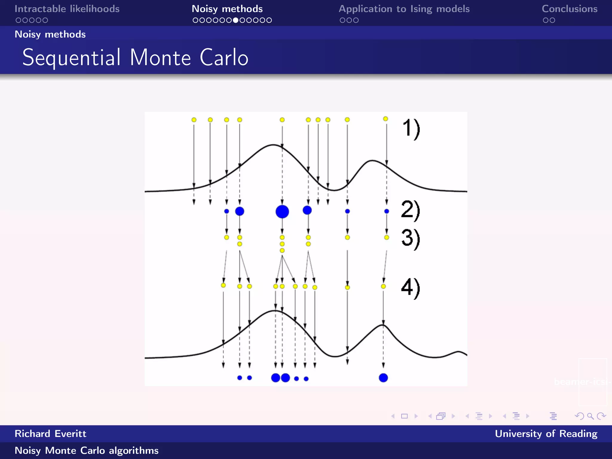
Noisy importance sampling and sequential Monte Carlo:
Everitt et al (2016).
Under some simplifying assumptions, noisy importance
sampling is more efficient (in terms of mean squared error)
compared to an exact-approximate algorithm if
1
P
Varq [w(θ)+b(θ)]+Eq[`σ2
θ ] +Eq[b(θ)]2
<
1
P
Varq [w(θ)]+Eq[´σ2
θ ] ,
where b(θ) > 0 is the bias of the noisy weights, `σ2
θ is the
variance of the noisy weights, ´σ2
θ is the variance of the
exact-approximate weights and
w(θ) :=
p(θ)γ(y|θ)
Z(θ)q(θ)
.
Richard Everitt University of Reading
Noisy Monte Carlo algorithms](https://image.slidesharecdn.com/everittparis-160712060244/75/Richard-Everitt-s-slides-19-2048.jpg)


The document discusses intractable likelihoods and the application of noisy Monte Carlo algorithms to Ising models. It explicates various methods for estimating likelihoods, including exact and approximate methods, and the challenges posed by doubly intractable distributions. Additionally, it highlights the effectiveness of noisy methods compared to traditional Monte Carlo techniques and presents empirical results related to their use in Ising models.


![[A]BCel : a presentation at ABC in Roma](https://cdn.slidesharecdn.com/ss_thumbnails/abcel-130530042650-phpapp02-thumbnail.jpg?width=640&height=640&fit=bounds)