Download as PDF, PPTX

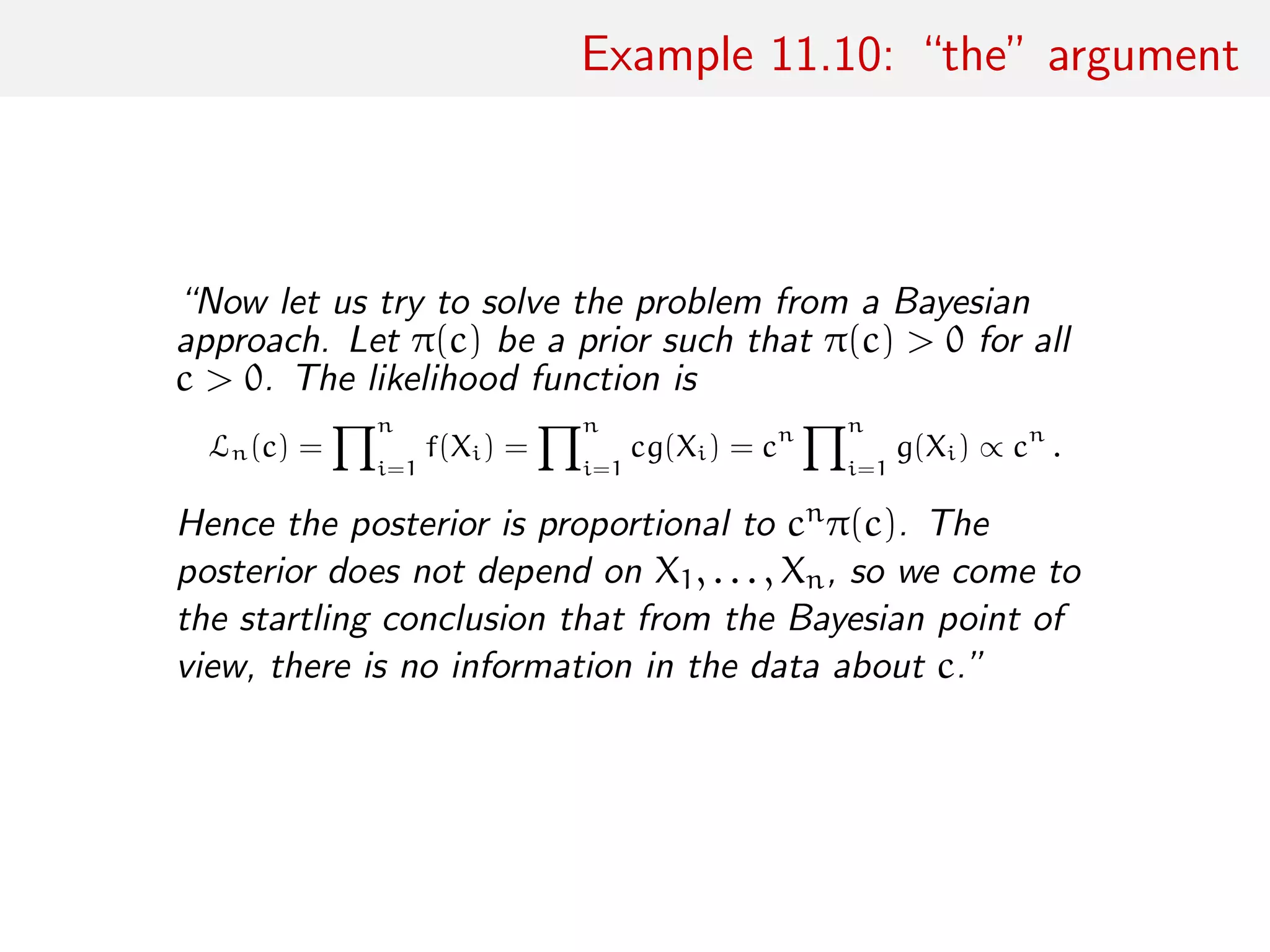
![c “Bayesians are slaves to the likelihood function”
• there is no likelihood function such as Ln(c) [since moving c
does not modify the sample]
• “there is no information in the data about c” but there is
about f
• not a statistical problem [at face value], rather a numerical
problem with many Monte Carlo solutions
• Monte Carlo methods are frequentist (LLN) and asymptotical
(as in large numbers)
• but use of probabilistic numerics brings uncertainty evaluation](https://image.slidesharecdn.com/isba-160607122654/75/Discussion-of-Persi-Diaconis-lecture-at-ISBA-2016-5-2048.jpg)
![a broader picture
• Larry’s problem somehow relates to the infamous harmonic
mean estimator issue
• highlight paradoxical differences between statistics and Monte
Carlo methods:
• statistics constrained by sample and its distribution
• Monte Carlo free to generate samples
• no best unbiased estimator or optimal solution in Monte Carlo
integration
• paradox of the fascinating “Bernoulli factory” problem, which
requires infinite sequence of Bernoullis
[Flegal & Herbei, 2012; Jacob & Thiery, 2015]
• highly limited range of parameters allowing for unbiased
estimation versus universal debiasing of converging sequences
[McLeish, 2011; Rhee & Glynn, 2012, 2013]](https://image.slidesharecdn.com/isba-160607122654/75/Discussion-of-Persi-Diaconis-lecture-at-ISBA-2016-6-2048.jpg)
![regression estimator
Given
Xij ∼ fi(x) = cihi(x)
with hi known and ci unknown (i = 1, . . . , k, j = 1, . . . , ni),
constants ci estimated by a “reverse logistic regression” based on
the quasi-likelihood
L(η) =
k
i=1
ni
j=1
log pi(xij, η)
with
pi(x, η) = exp{ηi}hi(x)
k
i=1
exp{ηi}hi(x)
[Anderson, 1972; Geyer, 1992]
Approximation
log ^ci = log ni/n − ^ηi](https://image.slidesharecdn.com/isba-160607122654/75/Discussion-of-Persi-Diaconis-lecture-at-ISBA-2016-8-2048.jpg)
![regression estimator
Given
Xij ∼ fi(x) = cihi(x)
with hi known and ci unknown (i = 1, . . . , k, j = 1, . . . , ni),
constants ci estimated by a “reverse logistic regression” based on
the quasi-likelihood
L(η) =
k
i=1
ni
j=1
log pi(xij, η)
with
pi(x, η) = exp{ηi}hi(x)
k
i=1
exp{ηi}hi(x)
[Anderson, 1972; Geyer, 1992]
Approximation
log ^ci = log ni/n − ^ηi](https://image.slidesharecdn.com/isba-160607122654/75/Discussion-of-Persi-Diaconis-lecture-at-ISBA-2016-9-2048.jpg)
![statistical framework?
Existence of a central limit theorem:
√
n (^ηn − η)
L
−→ Nk(0, B+
AB)
[Geyer, 1992; Doss & Tan, 2015]
• strong convergence properties
• asymptotic approximation of the precision
• connection with bridge sampling and auxiliary model [mixture]
• ...but nothing statistical there [no estimation]
• which optimality? [weights unidentifiable]
[Kong et al., 2003; Chopin & Robert, 2011]](https://image.slidesharecdn.com/isba-160607122654/75/Discussion-of-Persi-Diaconis-lecture-at-ISBA-2016-10-2048.jpg)
![statistical framework?
Existence of a central limit theorem:
√
n (^ηn − η)
L
−→ Nk(0, B+
AB)
[Geyer, 1992; Doss & Tan, 2015]
• strong convergence properties
• asymptotic approximation of the precision
• connection with bridge sampling and auxiliary model [mixture]
• ...but nothing statistical there [no estimation]
• which optimality? [weights unidentifiable]
[Kong et al., 2003; Chopin & Robert, 2011]](https://image.slidesharecdn.com/isba-160607122654/75/Discussion-of-Persi-Diaconis-lecture-at-ISBA-2016-11-2048.jpg)
![partition function and maximum likelihood
For parametric family
f(x; θ) = p(x; θ)/Z(θ)
• normalising constant Z(θ) also called partition function
• ...if normalisation possible
• essential part of inference
• estimation by score matching [matching scores of model and
data]
• ...and by noise-contrastive estimation [generalised Charlie’s
regression]
[Gutmann & Hyv¨arinen, 2012, 2015]](https://image.slidesharecdn.com/isba-160607122654/75/Discussion-of-Persi-Diaconis-lecture-at-ISBA-2016-12-2048.jpg)
![partition function and maximum likelihood
For parametric family
f(x; θ) = p(x; θ)/Z(θ)
Generic representation with auxiliary data y from known
distribution fy and regression function
h(u; θ) = 1 +
nx
ny
exp(−G(u; θ))
−1
Objective function
J(θ) =
nx
i=1
log h(xi; θ) +
ny
i=1
log{1 − h(yi; θ)}
that can be maximised with no normalising constant
[Gutmann & Hyv¨arinen, 2012, 2015]](https://image.slidesharecdn.com/isba-160607122654/75/Discussion-of-Persi-Diaconis-lecture-at-ISBA-2016-13-2048.jpg)
![Xiao-Li’s MLE
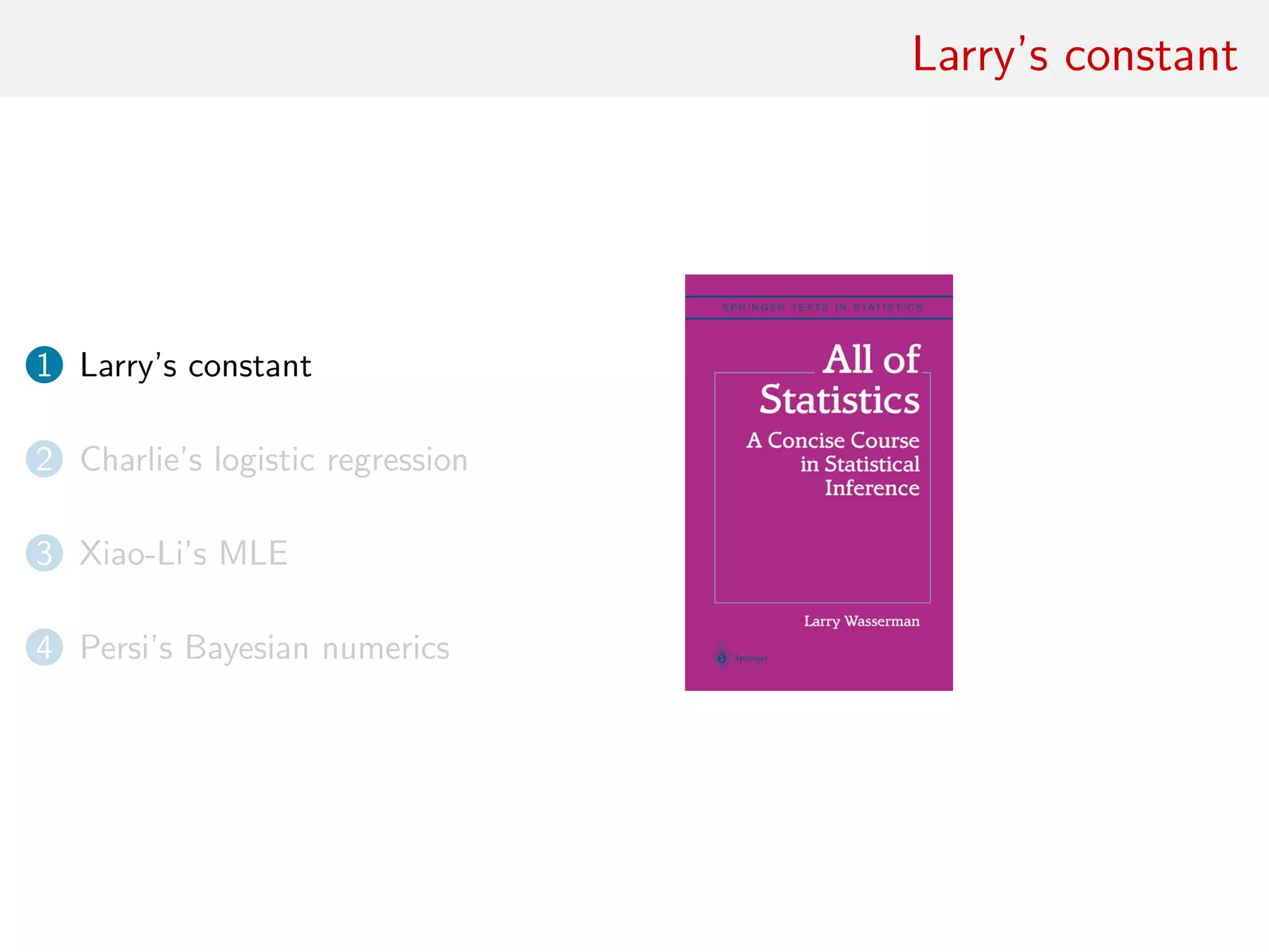
1 Larry’s constant
2 Charlie’s logistic regression
3 Xiao-Li’s MLE
4 Persi’s Bayesian numerics
[Meng, 2011, IRCEM]](https://image.slidesharecdn.com/isba-160607122654/75/Discussion-of-Persi-Diaconis-lecture-at-ISBA-2016-14-2048.jpg)
![Xiao-Li’s MLE
“The task of estimating an integral by Monte Carlo
methods is formulated as a statistical model using
simulated observations as data.
The difficulty in this exercise is that we ordinarily have
at our disposal all of the information required (..) but
we choose to ignore some (...) for simplicity or
computational feasibility.”
[Kong, McCullagh, Meng, Nicolae & Tan, 2003]](https://image.slidesharecdn.com/isba-160607122654/75/Discussion-of-Persi-Diaconis-lecture-at-ISBA-2016-15-2048.jpg)
![Xiao-Li’s MLE
“Our proposal is to use a semiparametric statistical
model that makes explicit what information is ignored
(...) The parameter space in this model is a set of
measures on the sample space (...) None-the-less,
from simulated data the base-line measure can be
estimated by maximum likelihood, and the required
integrals computed by a simple formula previously
derived by Geyer.”
[Kong, McCullagh, Meng, Nicolae & Tan, 2003]](https://image.slidesharecdn.com/isba-160607122654/75/Discussion-of-Persi-Diaconis-lecture-at-ISBA-2016-16-2048.jpg)
![Xiao-Li’s MLE
“By contrast with Geyer’s retrospective likelihood, a
correct estimate of simulation error is available
directly from the Fisher information. The principal
advantage of the semiparametric model is that
variance reduction techniques are associated with
submodels in which the maximum likelihood estimator
in the submodel may have substantially smaller
variance.”
[Kong, McCullagh, Meng, Nicolae & Tan, 2003]
(c.) Rachel2002](https://image.slidesharecdn.com/isba-160607122654/75/Discussion-of-Persi-Diaconis-lecture-at-ISBA-2016-17-2048.jpg)
![Xiao-Li’s MLE
“At first glance, the problem appears to be an exercise in calculus
or numerical analysis, and not amenable to statistical formulation”
• use of Fisher information
• non-parametric MLE based on
simulations
• comparison of sampling
schemes through variances
• Rao–Blackwellised
improvements by invariance
constraints [Meng, 2011, IRCEM]](https://image.slidesharecdn.com/isba-160607122654/75/Discussion-of-Persi-Diaconis-lecture-at-ISBA-2016-18-2048.jpg)
![reverse logistic regression
1 Larry’s constant
2 Charlie’s logistic regression
3 Xiao-Li’s MLE
4 Persi’s Bayesian numerics [P. Diaconis, 1988]](https://image.slidesharecdn.com/isba-160607122654/75/Discussion-of-Persi-Diaconis-lecture-at-ISBA-2016-19-2048.jpg)
![My uncertainties
• answer to the zero variance estimator
• significance of a probability statement about a mathematical
constant [other than epistemic]
• posterior in functional spaces mostly reflect choice of prior
rather than information
• big world versus small worlds debate
[Robbins & Wasserman, 2000]
• possible incoherence of Bayesian inference in functional spaces
• unavoidable recourse to (and impact of) Bayesian prior
modelling](https://image.slidesharecdn.com/isba-160607122654/75/Discussion-of-Persi-Diaconis-lecture-at-ISBA-2016-22-2048.jpg)
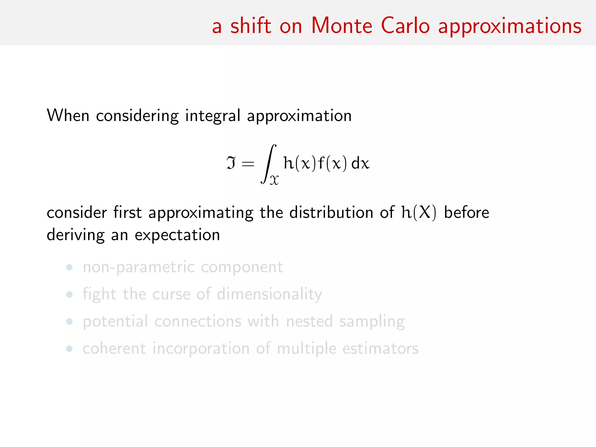
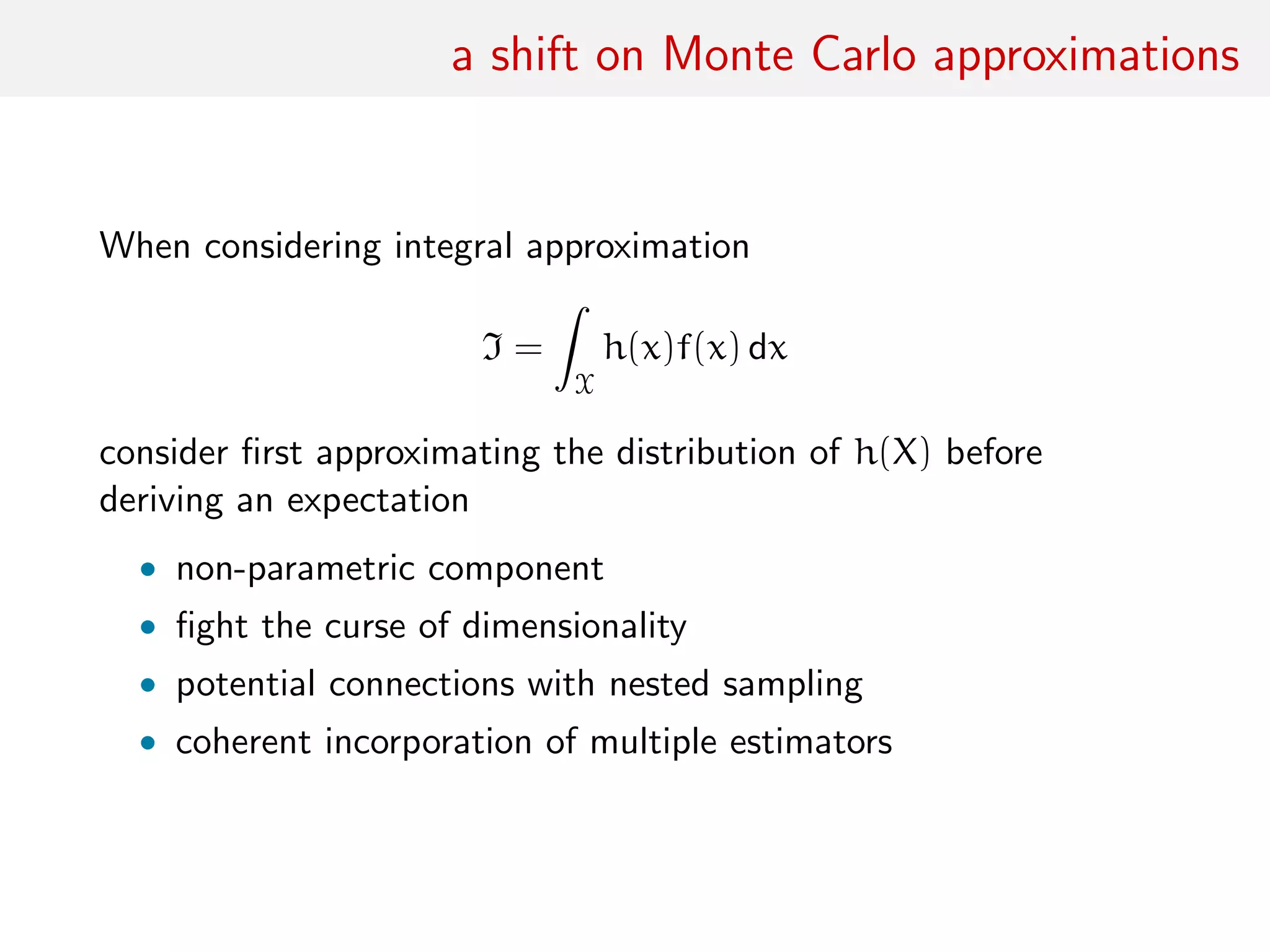

This document discusses Monte Carlo methods for numerical integration and estimating normalizing constants. It summarizes several approaches: estimating normalizing constants using samples; reverse logistic regression for estimating constants in mixtures; Xiao-Li's maximum likelihood formulation for Monte Carlo integration; and Persi's probabilistic numerics which provide uncertainties for numerical calculations. The document advocates first approximating the distribution of an integrand before estimating its expectation to incorporate non-parametric information and account for multiple estimators.